Navier-Stokes: Cavity Flow

Cavity flow can be considered a canonical solution for the Navier-Stokes, given how well the solution to this problem is known. In this exampled it is solved for the case of \(Re = 10\), since that allows for quick convergence on a fairly coarse grid.

import numpy as np
import pyvista as pv
import rmsh
from mfv2d import (
    BoundaryCondition2DSteady,
    KFormSystem,
    KFormUnknown,
    Mesh2D,
    SolverSettings,
    SystemSettings,
    TimeSettings,
    UnknownFormOrder,
    solve_system_2d,
)

Setup

Since there’s no manufactured solution, the only necessary setup is the boundary velocity, which should be 2 on the top side of the mesh and zero elsewhere. The reason for it being 2 is because the domain length is also 2.

RE = 1e1


def boundary_velocty(x, y):
    """Exact velocity solution."""
    vx = 2 * (y == 1) + 0 * x
    vy = 0 * (x + y)
    return np.stack((vx, vy), axis=-1)

System Setup

System is set up the same as with the steady example of Navier-Stokes, with the only difference being the weak pressure boundary conditions not being included, due to the fact that the strong boundary conditions on the normal velocity mean that they would not be used either way.

pre = KFormUnknown("pre", UnknownFormOrder.FORM_ORDER_2)
w_pre = pre.weight
vel = KFormUnknown("vel", UnknownFormOrder.FORM_ORDER_1)
w_vel = vel.weight
vor = KFormUnknown("vor", UnknownFormOrder.FORM_ORDER_0)
w_vor = vor.weight

system = KFormSystem(
    w_vor.derivative * vel - w_vor * vor == w_vor ^ boundary_velocty,
    # No weak BC for pressure, since normal velocity is given
    (1 / RE) * (w_vel * vor.derivative) + w_vel.derivative * pre
    == -(w_vel * (vel ^ (~vor))),
    w_pre * vel.derivative == 0,
    sorting=lambda f: f.order,
)
print(system)

N = 6
P = 3

n1 = N
n2 = N

rect_mesh, rx, ry = rmsh.create_elliptical_mesh(
    rmsh.MeshBlock(
        label=None,
        bottom=rmsh.BoundaryCurve.from_knots(n1, (-1, -1), (+1, -1)),
        right=rmsh.BoundaryCurve.from_knots(n2, (+1, -1), (+1, +1)),
        top=rmsh.BoundaryCurve.from_knots(n1, (+1, +1), (-1, +1)),
        left=rmsh.BoundaryCurve.from_knots(n2, (-1, +1), (-1, -1)),
    )
)
assert rx < 1e-6, ry < 1e-6

mesh = Mesh2D(
    P,
    np.stack((rect_mesh.pos_x, rect_mesh.pos_y), axis=-1),
    rect_mesh.lines + 1,
    rect_mesh.surfaces,
)

solutions, stats = solve_system_2d(
    mesh,
    SystemSettings(
        system,
        [BoundaryCondition2DSteady(vel, mesh.boundary_indices, boundary_velocty)],
        [(0.0, pre)],
    ),
    solver_settings=SolverSettings(
        maximum_iterations=100,
        absolute_tolerance=1e-10,
        relative_tolerance=0,
    ),
    time_settings=TimeSettings(dt=5, nt=20, time_march_relations={w_vel: vel}),
    print_residual=False,
    recon_order=25,
)
print(stats)

[vor(1*)]^T  ([           -1 * M(1) | (E(2, 1))^T @ M(1) |                  0]  [vor(0)]   [<vor, boundary_velocty>])   [vor(1*)]^T  ([                              0 |                        0 | 0]  [vor(0)]
[vel(2*)]    ([0.1 * M(2) @ E(2, 1) |                  0 | (E(3, 2))^T @ M(2)]  [vel(1)] = [                       ]) + [vel(2*)]    ([-1 * M(2) @ M(2, 3; vel) @ M(1) | -1 * M(2) @ N(2, 3; vor) | 0]  [vel(1)]
[pre(3*)]    ([                   0 |     M(3) @ E(3, 2) |                  0]  [pre(2)]   [                      0])   [pre(3*)]    ([                              0 |                        0 | 0]  [pre(2)]
SolutionStatistics(element_orders={3: 50}, n_total_dofs=1550, n_leaf_dofs=1225, n_lagrange=325, n_elems=25, n_leaves=25, iter_history=array([20, 24, 20, 22, 20, 21, 20, 21, 20, 20, 20, 20, 20, 20, 20, 20, 20,
       20, 20, 20], dtype=uint32), residual_history=array([4.73040218e-11, 3.78859860e-11, 4.94556202e-11, 4.77373419e-11,
       6.63145788e-11, 4.92627328e-11, 6.85677765e-11, 4.04782319e-11,
       7.24523080e-11, 9.98627847e-11, 7.65691122e-11, 9.79617637e-11,
       7.69061897e-11, 9.11821313e-11, 7.17330223e-11, 8.28753177e-11,
       7.86609111e-11, 9.14862630e-11, 8.53559723e-11, 9.54867019e-11]))

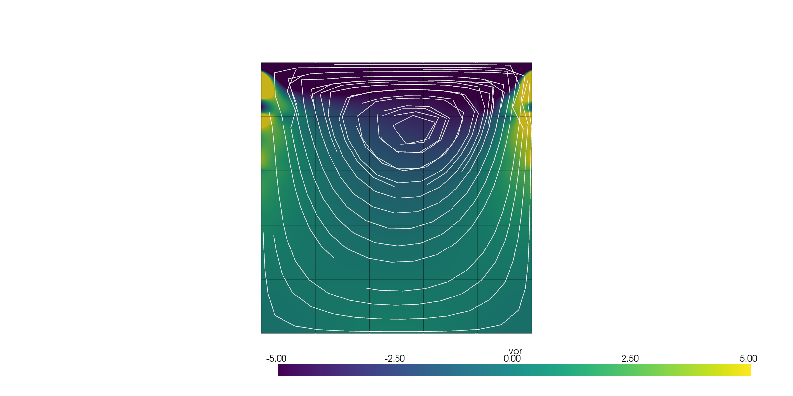
Plot Streamlines

Pyvista allows for very simple 2D streamline plots.

plotter = pv.Plotter(off_screen=True, shape=(1, 1), window_size=(1600, 800))

solution = solutions[-1]
solution.point_data[vel.label] = np.pad(solution.point_data[vel.label], ((0, 0), (0, 1)))
plotter.add_mesh(solution.copy(), scalars=vor.label, clim=(-5, +5))
plotter.add_mesh(solution.extract_all_edges(), color="black")
plotter.add_mesh(
    solution.streamlines_evenly_spaced_2D(
        vectors=vel.label,
        step_length=0.3,
        start_position=(0, 0, 0),
        separating_distance=0.2,
        separating_distance_ratio=0.1,
        compute_vorticity=False,
    ),
    scalars=None,
    show_scalar_bar=False,
    color="white",
)
plotter.view_xy()