Note
Go to the end to download the full example code.
Post-Solver p-Refinement#
As mentioned in Poisson Equation with Local Refinement example, refinement can be done “post-solver” as well. This means that mesh refinement is performed after the solver finishes running. This does not change the computed solution, but allows for next solve to be more accurate, if repeated.
The setup for the run is the same as one in Poisson Equation with Local Refinement, so it will be only briefly mentioned.
import numpy as np
import numpy.typing as npt
import pyvista as pv
import rmsh
from matplotlib import pyplot as plt
from matplotlib.collections import PolyCollection
from mfv2d import (
    BoundaryCondition2DSteady,
    KFormSystem,
    KFormUnknown,
    Mesh,
    RefinementLimitElementCount,  # Need a refinement limit
    RefinementSettings,  # Need refinement settings
    SystemSettings,
    UnknownFormOrder,
    mesh_create,
    solve_system_2d,
)
Manufactured Solution#
Manufactured solution in this case is intentionally more localized. It is given by equation (1). Since the solution is very localized, this example should serve as a good indicator for how local refinement improves refinement efficiency.
def s(t: npt.NDArray[np.float64], r: float, t0: float) -> npt.NDArray[np.floating]:
    """Compute source term."""
    return np.exp(-r * (t - t0) ** 2)


def dsdt(t: npt.NDArray[np.float64], r: float, t0: float) -> npt.NDArray[np.floating]:
    """Compute derivative source term."""
    return -2 * r * (t - t0) * np.exp(-r * (t - t0) ** 2)


def d2sdt2(t: npt.NDArray[np.float64], r: float, t0: float) -> npt.NDArray[np.floating]:
    """Compute second derivative source term."""
    return 2 * r * (2 * r * (t - t0) ** 2 - 1) * np.exp(-r * (t - t0) ** 2)


def u_exact(x: npt.NDArray[np.float64], y: npt.NDArray[np.float64]):
    """Exact solution."""
    return s(x, 10.0, 0.75) * s(y, 10.0, 0.75)


def q_exact(x: npt.NDArray[np.float64], y: npt.NDArray[np.float64]):
    """Exact curl of solution."""
    return np.stack(
        (
            s(x, 10.0, 0.75) * dsdt(y, 10.0, 0.75),
            -dsdt(x, 10.0, 0.75) * s(y, 10.0, 0.75),
        ),
        axis=-1,
    )


def source_exact(x: npt.NDArray[np.float64], y: npt.NDArray[np.float64]):
    """Exact heat flux divergence."""
    return s(x, 10.0, 0.75) * d2sdt2(y, 10.0, 0.75) + d2sdt2(x, 10.0, 0.75) * s(
        y, 10.0, 0.75
    )


q = KFormUnknown("q", UnknownFormOrder.FORM_ORDER_1)
p = q.weight
u = KFormUnknown("u", UnknownFormOrder.FORM_ORDER_0)
v = u.weight

system = KFormSystem(
    v.derivative * u.derivative == -(v * source_exact) + (v ^ q_exact),
    p * u.derivative - p * q == 0,
    sorting=lambda f: f.order,
)
print(system)
[u(0*)]^T  ([(E(1, 0))^T @ M(0) @ E(1, 0) |         0]  [u(0)]   [-1 * <u, source_exact> + <u, q_exact>])
[q(1*)]    ([              M(1) @ E(1, 0) | -1 * M(1)]  [q(1)] = [                                    0])
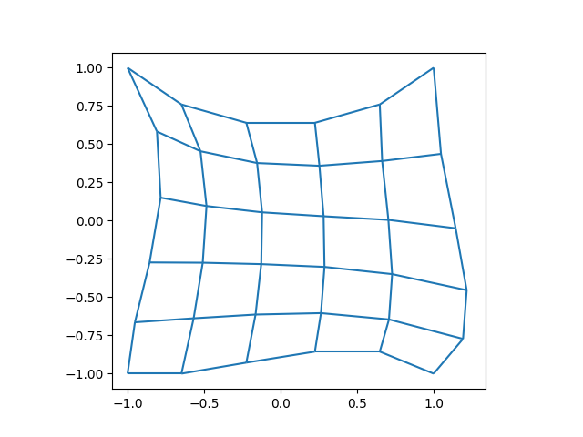
Initial Mesh#
The initial mesh is the same as for the pre-solver refinement example.
N = 6
n1 = N
n2 = N
m, rx, ry = rmsh.create_elliptical_mesh(
rmsh.MeshBlock(
None,
rmsh.BoundaryCurve.from_knots(
n1, (-1, -1), (-0.5, -1.1), (+0.5, -0.6), (+1, -1)
), # bottom
rmsh.BoundaryCurve.from_knots(
n2, (+1, -1), (+1.5, -0.7), (+1, 0.0), (+1, +1)
), # right
rmsh.BoundaryCurve.from_knots(
n1, (+1, +1), (0.5, 0.5), (-0.5, 0.5), (-1, +1)
), # top
rmsh.BoundaryCurve.from_knots(
n2, (-1, +1), (-0.5, 0.33), (-1, -0.5), (-1, -1)
), # left
)
)
assert rx < 1e-6 and ry < 1e-6
# Show the mesh for the first time.
fig, ax = plt.subplots(1, 1)
xlim, ylim = m.plot(ax)
ax.set_xlim(1.1 * xlim[0], 1.1 * xlim[1])
ax.set_ylim(1.1 * ylim[0], 1.1 * ylim[1])
ax.set_aspect("equal")
plt.show()
pval = 3 # Test polynomial order
mesh = mesh_create(pval, np.stack((m.pos_x, m.pos_y), axis=-1), m.lines + 1, m.surfaces)
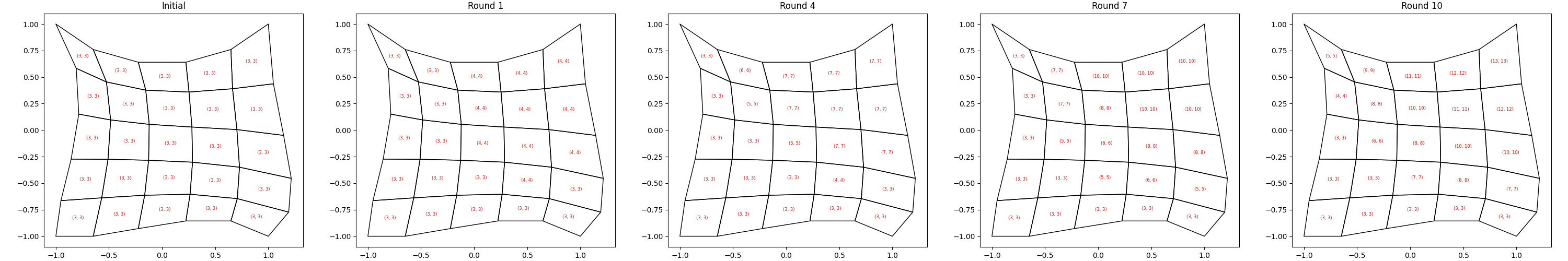
def plot_mesh_comparisons(*meshes: tuple[str, Mesh]) -> None:
"""Plot one or more meshes with given titles."""
fig, axes = plt.subplots(1, len(meshes), figsize=(6 * len(meshes), 5))
for ax, (title, mesh) in zip(axes, meshes, strict=True):
vertices = [mesh.get_leaf_corners(idx) for idx in mesh.get_leaf_indices()]
ax.add_collection(PolyCollection(vertices, facecolors="none", antialiased=True))
for idx, quad in zip(mesh.get_leaf_indices(), vertices):
ax.text(
*np.mean(quad, axis=0),
str(mesh.get_leaf_orders(idx)),
ha="center",
va="center",
color="red",
fontsize=6,
)
ax.autoscale()
ax.set(aspect="equal", title=title)
fig.tight_layout()
plt.show()
Refinement Settings#
Post-solver refinement is controlled with the RefinementSettings type.
The main setting is it is the error_calculation_function, which should be
set to a function which computes two values:
Error in some norm or semi-norm,
Cost of h-refinement in that norm,
If the ratio of the cost of h-refinement and error is bellow the value specified
as the h_refinement_ratio, then the element will be h-refined. Otherwise it
will be a candidate for p-refinement.
For this example, the error measure is exact \(L^2\) norm (since the
manufactured solution is known), and measure of h-refinement cost is given as just
an arbitrary constant, since h_refinement_ratio = 0, meaning it will never happen.
To specify when the refinement should stop, refinement_limit should be given.
In this case, RefinementLimitElementCount is used to specify that at
either 10 elements or 100 % of the elements, whichever is lower, can be refined
each iteration.
def error_calc_function(
    x: npt.NDArray[np.float64],
    y: npt.NDArray[np.float64],
    w: npt.NDArray[np.float64],
    **kwargs,
) -> tuple[float, float]:
    """Compute L2 error "estimate" and H1 refinement cost."""
    assert len(kwargs) == 1
    u = kwargs["u"]
    real_u = u_exact(x, y)
    err = (real_u - u) ** 2 * w
    return np.sum(err), 1.0


refinement_settings = RefinementSettings(
    required_forms=[u],  # Required by the error function
    error_calculation_function=error_calc_function,  # The error function
    h_refinement_ratio=0,  # H-refinement when ratio of h-cost and error less than this
    refinement_limit=RefinementLimitElementCount(1.0, 10),  # When to stop refining
    report_error_distribution=True,  # Print error distribution to terminal
    report_order_distribution=True,  # Print element order distribution to terminal
)
Iteratively Refining the Mesh#
Here the mesh is iteratively refined number of times, as given by N_ROUNDS.
For each round, a plot of error and element orders is shown.
N_ROUNDS = 10
system_settings = SystemSettings(
    system=system,
    boundary_conditions=[BoundaryCondition2DSteady(u, mesh.boundary_indices, u_exact)],
)

results = [("Initial", mesh)]
errors_local: list[tuple[int, float]] = list()
plotter = pv.Plotter(off_screen=True, window_size=(1600, 900), shape=(1, 2))
plotter.open_gif("direct-poisson-refinement-post-p.gif", fps=1)

for i_round in range(N_ROUNDS):
    base_mesh = mesh
    solutions, statistics, mesh = solve_system_2d(
        mesh,
        system_settings=system_settings,
        refinement_settings=refinement_settings,
        recon_order=15,
    )

    solution = solutions[-1]
    u_computed = solution.point_data[u.label]
    u_real = u_exact(solution.points[:, 0], solution.points[:, 1])
    l2_err2 = (u_real - u_computed) ** 2
    solution.point_data["l2_error2"] = l2_err2

    plotter.subplot(0, 0)
    plotter.add_mesh(
        solution,
        scalars="l2_error2",
        log_scale=True,
        label="$L^2$ error",
        clim=(1e-20, 1e-4),
        name="solution",
    )
    plotter.add_mesh(
        solution.extract_all_edges(), scalars=None, color="black", name="boundaries"
    )
    plotter.view_xy()

    plotter.subplot(0, 1)
    sol = solution.copy()
    sol.cell_data["geometrical order"] = np.linalg.norm(
        [mesh.get_leaf_orders(ie) for ie in base_mesh.get_leaf_indices()], axis=-1
    ) / np.sqrt(2)
    plotter.add_mesh(sol, scalars="geometrical order", name="orders", clim=(1, 12))
    plotter.add_text(f"Round {i_round + 1:d}", name="title")
    plotter.view_xy()

    plotter.write_frame()

    results.append((f"Round {i_round + 1:d}", mesh))
    errors_local.append(
        (
            statistics.n_total_dofs,
            np.sqrt(solution.integrate_data().point_data["l2_error2"][0]),
        )
    )
plotter.close()
Initial mesh order distribution
============================================================
█
█
█
█
████████████████████████████████████████████████████████████
| | | | |
2.5 2.7 3.0 3.2 3.5
============================================================
Error estimate distribution
============================================================
█
█ █ █ █ █
█ █ █ █ █
█ ██ █ █ █ █ ██ █ ██ ███ █ █ █ █
████████████████████████████████████████████████████████████
| | | | |
10^(-13) 10^(-11) 10^(-8.3) 10^(-5.9) 10^(-3.6)
============================================================
Refined mesh order distribution
============================================================
█
█ █
█ █
█ █
████████████████████████████████████████████████████████████
| | | | |
3.0 3.2 3.5 3.7 4.0
============================================================
Initial mesh order distribution
============================================================
█
█ █
█ █
█ █
████████████████████████████████████████████████████████████
| | | | |
3.0 3.2 3.5 3.7 4.0
============================================================
Error estimate distribution
============================================================
█ █
█ █
█ █ █ █ █ ████ █ ███ █ █ █ █ █ █ █ ██ █
█ █ █ █ █ ████ █ ███ █ █ █ █ █ █ █ ██ █
████████████████████████████████████████████████████████████
| | | | |
10^(-16) 10^(-13) 10^(-11) 10^(-7.7) 10^(-4.9)
============================================================
Refined mesh order distribution
============================================================
█
█
█ █
█ █ █
████████████████████████████████████████████████████████████
| | | | |
3.0 3.5 4.0 4.5 5.0
============================================================
Initial mesh order distribution
============================================================
█
█
█ █
█ █ █
████████████████████████████████████████████████████████████
| | | | |
3.0 3.5 4.0 4.5 5.0
============================================================
Error estimate distribution
============================================================
█
█ █ █
█ █ █
█ █ ███ ███ ███ █ █ █ █ █ █ █ █ █ █
████████████████████████████████████████████████████████████
| | | | |
10^(-16) 10^(-14) 10^(-11) 10^(-8.9) 10^(-6.3)
============================================================
Refined mesh order distribution
============================================================
█
█
█ █
█ █ █ █
████████████████████████████████████████████████████████████
| | | | |
3.0 3.7 4.4 5.2 5.9
============================================================
Initial mesh order distribution
============================================================
█
█
█ █
█ █ █ █
████████████████████████████████████████████████████████████
| | | | |
3.0 3.7 4.4 5.2 5.9
============================================================
Error estimate distribution
============================================================
█ █
█ █ █
█ █ █
█ ██ █ ███ █ █ █ ██ █ █ █ █ █ █ █ █
████████████████████████████████████████████████████████████
| | | | |
10^(-18) 10^(-16) 10^(-13) 10^(-10) 10^(-7.6)
============================================================
Refined mesh order distribution
============================================================
█
█
█ █
█ █ █
████████████████████████████████████████████████████████████
| | | | |
3.0 3.9 4.9 5.9 6.9
============================================================
Initial mesh order distribution
============================================================
█
█
█ █
█ █ █
████████████████████████████████████████████████████████████
| | | | |
3.0 3.9 4.9 5.9 6.9
============================================================
Error estimate distribution
============================================================
█
█ █ █
█ █ █
█ █ █ ██ ██ █ ████████ ██ █ █ █
████████████████████████████████████████████████████████████
| | | | |
10^(-21) 10^(-18) 10^(-15) 10^(-12) 10^(-9.3)
============================================================
Refined mesh order distribution
============================================================
█
█
█ █
█ █ █ █
████████████████████████████████████████████████████████████
| | | | |
3.0 4.2 5.4 6.7 7.9
============================================================
Initial mesh order distribution
============================================================
█
█
█ █
█ █ █ █
████████████████████████████████████████████████████████████
| | | | |
3.0 4.2 5.4 6.7 7.9
============================================================
Error estimate distribution
============================================================
█
█ █ ███
█ █ ███
█ █ █ █ █ █ ██ █ █████ █ █ █ █ █
████████████████████████████████████████████████████████████
| | | | |
10^(-21) 10^(-19) 10^(-16) 10^(-13) 10^(-10)
============================================================
Refined mesh order distribution
============================================================
█
█
█ █ █
█ █ █ █ █
████████████████████████████████████████████████████████████
| | | | |
3.0 4.4 5.9 7.4 8.9
============================================================
Initial mesh order distribution
============================================================
█
█
█ █ █
█ █ █ █ █
████████████████████████████████████████████████████████████
| | | | |
3.0 4.4 5.9 7.4 8.9
============================================================
Error estimate distribution
============================================================
█
█ █
█ █ █ █
█ █ █ ███ █ █ ██████ ███ █
████████████████████████████████████████████████████████████
| | | | |
10^(-22) 10^(-20) 10^(-17) 10^(-15) 10^(-12)
============================================================
Refined mesh order distribution
============================================================
█
█
█ █
█ █ █ █ █ █
████████████████████████████████████████████████████████████
| | | | |
3.0 4.6 6.4 8.1 9.9
============================================================
Initial mesh order distribution
============================================================
█
█
█ █
█ █ █ █ █ █
████████████████████████████████████████████████████████████
| | | | |
3.0 4.6 6.4 8.1 9.9
============================================================
Error estimate distribution
============================================================
█
█ █ █ █ █
█ █ █ █ █
█ ██ █ █ █ █ ██ ██ ███ ███ █ █
████████████████████████████████████████████████████████████
| | | | |
10^(-23) 10^(-21) 10^(-19) 10^(-16) 10^(-13)
============================================================
Refined mesh order distribution
============================================================
█
█
█
█ █ █ █ █ █
████████████████████████████████████████████████████████████
| | | | |
3.0 4.9 6.9 8.9 10.9
============================================================
Initial mesh order distribution
============================================================
█
█
█
█ █ █ █ █ █
████████████████████████████████████████████████████████████
| | | | |
3.0 4.9 6.9 8.9 10.9
============================================================
Error estimate distribution
============================================================
█
██████
██████
█ ██ █ ██ █ █ ██ ███████ █
████████████████████████████████████████████████████████████
| | | | |
10^(-24) 10^(-22) 10^(-20) 10^(-17) 10^(-15)
============================================================
Refined mesh order distribution
============================================================
█
█
█ █
█ █ █ █ █ █
████████████████████████████████████████████████████████████
| | | | |
3.0 5.1 7.3 9.6 11.8
============================================================
Initial mesh order distribution
============================================================
█
█
█ █
█ █ █ █ █ █
████████████████████████████████████████████████████████████
| | | | |
3.0 5.1 7.3 9.6 11.8
============================================================
Error estimate distribution
============================================================
█ █ █
█ █ █ █ █
█ █ █ █ █
█ ██ █ █ ██ █ ███ █ █ █ ██ █
████████████████████████████████████████████████████████████
| | | | |
10^(-23) 10^(-22) 10^(-20) 10^(-18) 10^(-16)
============================================================
Refined mesh order distribution
============================================================
█
█
█ █ █
█ █ █ █ █ █
████████████████████████████████████████████████████████████
| | | | |
3.0 5.3 7.8 10.3 12.8
============================================================
Comparison of All Meshes#
Here the meshes are compared to one another.
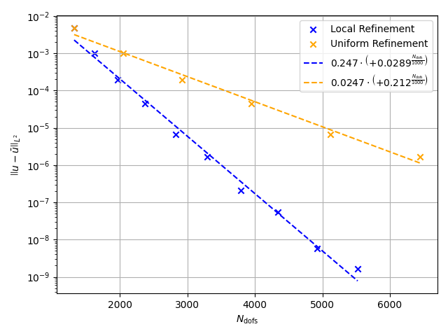
Error Evolution#
Error evolution of the post-refined mesh is presented here in contrast to uniform refinement.
errors_uniform: list[tuple[int, float]] = list()

for pval in range(3, 9):
    mesh = mesh_create(
        pval, np.stack((m.pos_x, m.pos_y), axis=-1), m.lines + 1, m.surfaces
    )
    solutions, statistics, _ = solve_system_2d(
        mesh,
        system_settings=system_settings,
        refinement_settings=None,
        recon_order=15,
    )
    solution = solutions[-1]
    u_computed = solution.point_data[u.label]
    u_real = u_exact(solution.points[:, 0], solution.points[:, 1])
    l2_err2 = (u_real - u_computed) ** 2
    solution.point_data["l2_error2"] = l2_err2
    errors_uniform.append(
        (
            statistics.n_total_dofs,
            np.sqrt(solution.integrate_data().point_data["l2_error2"][0]),
        )
    )

fig, ax = plt.subplots()

el = np.array(errors_local)
eu = np.array(errors_uniform)

kl1, kl0 = np.polyfit(el[:, 0] / 1000, np.log(el[:, 1]), 1)
kl1, kl0 = np.exp(kl1), np.exp(kl0)
ku1, ku0 = np.polyfit(eu[:, 0] / 1000, np.log(eu[:, 1]), 1)
ku1, ku0 = np.exp(ku1), np.exp(ku0)

ax.scatter(el[:, 0], el[:, 1], label="Local Refinement", marker="x", color="blue")
ax.scatter(eu[:, 0], eu[:, 1], label="Uniform Refinement", marker="x", color="orange")
ax.plot(
    el[:, 0],
    kl0 * kl1 ** (el[:, 0] / 1000),
    label=f"${kl0:.3g} \\cdot \\left({{{kl1:+.3g}}}^{{\\frac{{N_\\mathrm{{dofs}}}}"
    f"{{1000}}}}\\right)$",
    color="blue",
    linestyle="dashed",
)
ax.plot(
    eu[:, 0],
    ku0 * ku1 ** (eu[:, 0] / 1000),
    label=f"${ku0:.3g} \\cdot \\left({{{ku1:+.3g}}}^{{\\frac{{N_\\mathrm{{dofs}}}}"
    f"{{1000}}}}\\right)$",
    color="orange",
    linestyle="dashed",
)
ax.grid()
ax.legend()
ax.set(
    xlabel="$N_\\mathrm{dofs}$",
    ylabel="$\\left|\\left| u - \\bar{u} \\right|\\right|_{L^2}$",
    yscale="log",
)
fig.tight_layout()

plt.show()
Total running time of the script: (0 minutes 12.889 seconds)