Poisson Equation with Local Refinement

One of key features of mfv2d is the ability to locally refine the mesh with both hierarchical refinement (divide elements) or with polynomial refinement (increase order of elements).

This examples is otherwise identical to Poisson Equation in the Direct Formulation, where the direct Poisson is solved in a straight-forward manner. As such, only text and comments added to the code are pertaining to features not used in that one.

import numpy as np
import numpy.typing as npt
import pyvista as pv
import rmsh
from matplotlib import pyplot as plt
from matplotlib.collections import PolyCollection
from mfv2d import (
    BoundaryCondition2DSteady,
    KFormSystem,
    KFormUnknown,
    Mesh,
    SolverSettings,
    SystemSettings,
    UnknownFormOrder,
    mesh_create,
    solve_system_2d,
)


def u_exact(x: npt.NDArray[np.float64], y: npt.NDArray[np.float64]):
    """Exact solution."""
    return 2 * np.cos(np.pi / 2 * x) * np.cos(np.pi / 2 * y) + 5


def q_exact(x: npt.NDArray[np.float64], y: npt.NDArray[np.float64]):
    """Exact curl of solution."""
    return np.stack(
        (
            -np.pi * np.cos(np.pi / 2 * x) * np.sin(np.pi / 2 * y),
            np.pi * np.sin(np.pi / 2 * x) * np.cos(np.pi / 2 * y),
        ),
        axis=-1,
    )


def source_exact(x: npt.NDArray[np.floating], y: npt.NDArray[np.floating]):
    """Exact heat flux divergence."""
    return -(np.pi**2) * np.cos(np.pi / 2 * x) * np.cos(np.pi / 2 * y)


q = KFormUnknown("q", UnknownFormOrder.FORM_ORDER_1)
p = q.weight
u = KFormUnknown("u", UnknownFormOrder.FORM_ORDER_0)
v = u.weight

system = KFormSystem(
    v.derivative * u.derivative == -(v * source_exact) + (v ^ q_exact),
    p * u.derivative - p * q == 0,
    sorting=lambda f: f.order,
)
print(system)

N = 6
n1 = N
n2 = N


m, rx, ry = rmsh.create_elliptical_mesh(
    rmsh.MeshBlock(
        None,
        rmsh.BoundaryCurve.from_knots(
            n1, (-1, -1), (-0.5, -1.1), (+0.5, -0.6), (+1, -1)
        ),  # bottom
        rmsh.BoundaryCurve.from_knots(
            n2, (+1, -1), (+1.5, -0.7), (+1, 0.0), (+1, +1)
        ),  # right
        rmsh.BoundaryCurve.from_knots(
            n1, (+1, +1), (0.5, 0.5), (-0.5, 0.5), (-1, +1)
        ),  # top
        rmsh.BoundaryCurve.from_knots(
            n2, (-1, +1), (-0.5, 0.33), (-1, -0.5), (-1, -1)
        ),  # left
    )
)
assert rx < 1e-6 and ry < 1e-6

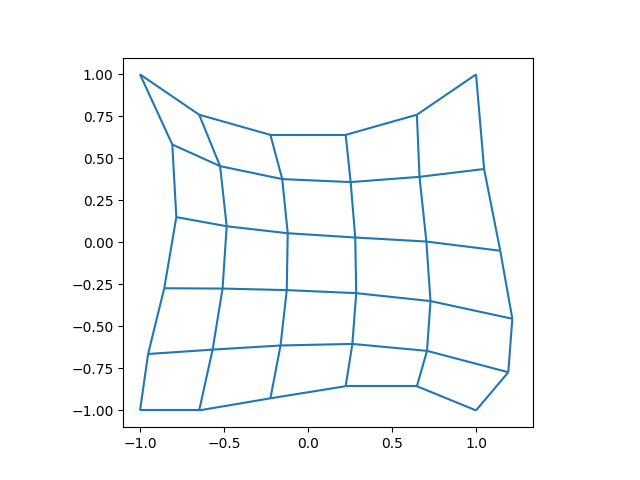
# Show the mesh for the first time.
fig, ax = plt.subplots(1, 1)
xlim, ylim = m.plot(ax)
ax.set_xlim(1.1 * xlim[0], 1.1 * xlim[1])
ax.set_ylim(1.1 * ylim[0], 1.1 * ylim[1])
ax.set_aspect("equal")
plt.show()

pval = 1  # Test polynomial order
mesh = mesh_create(pval, np.stack((m.pos_x, m.pos_y), axis=-1), m.lines + 1, m.surfaces)

[u(0*)]^T  ([(E(1, 0))^T @ M(0) @ E(1, 0) |         0]  [u(0)]   [-1 * <u, source_exact> + <u, q_exact>])
[q(1*)]    ([              M(1) @ E(1, 0) | -1 * M(1)]  [q(1)] = [                                    0])

Refinement Settings

Refinement can be done in two ways - pre-solver refinement and post-solver refinement. For pre-solver refinement, the choice of which elements are hierarchically refined is based soley on geometrical and topological data. This is quite clearly because no solution has been computed yet.

Pre-solver refinement is facilitated by methods mfv2d._mfv2d.Mesh.split_depth_first() and mfv2d._mfv2d.Mesh.split_breath_first(). Both accept a predicate function they evaluate for each element that could be refined, until a desired depth of refinement is reached, or all leaf elements have been checked already. The difference between the two is the order in which they examine leaves. Post-solver refinement is more involved, so it won’t me discussed here in more detail.

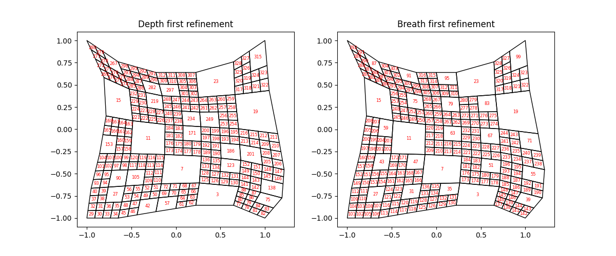
The example bellow shows how the refinement will differ if first 3 out of 4 elements that are checked are refined. Note that this is just for illustrative purposes and that in a more realistic case for pre-solver refinement, geometry of each element could be checked through the mfv2d._mfv2d.Mesh.get_leaf_corners().

def division_predicate(m: Mesh, ie: int, counter: list[int]):
    """Test division predicate."""
    counter[0] += 1
    cnt = counter[0]
    if (cnt & 3) != 0:
        orders = m.get_leaf_orders(ie)
        return orders, orders, orders, orders
    return None


counter = [0]
depth_mesh = mesh.split_depth_first(2, division_predicate, counter)

# Reset the counter
counter = [0]
breath_mesh = mesh.split_breath_first(2, division_predicate, counter)


fig, (ax1, ax2) = plt.subplots(1, 2, figsize=(12, 5))

vertices_depth = [
    depth_mesh.get_leaf_corners(idx) for idx in depth_mesh.get_leaf_indices()
]
ax1.add_collection(
    PolyCollection(
        vertices_depth,
        facecolors="none",
        antialiased=True,
    )
)
for idx, quad in zip(depth_mesh.get_leaf_indices(), vertices_depth):
    ax1.text(
        *np.mean(quad, axis=0),
        str(idx),
        ha="center",
        va="center",
        color="red",
        fontsize=6,
    )
ax1.autoscale()
ax1.set(aspect="equal", title="Depth first refinement")

vertices_breath = [
    breath_mesh.get_leaf_corners(idx) for idx in breath_mesh.get_leaf_indices()
]
ax2.add_collection(
    PolyCollection(
        vertices_breath,
        facecolors="none",
        antialiased=True,
    )
)
for idx, quad in zip(breath_mesh.get_leaf_indices(), vertices_breath):
    ax2.text(
        *np.mean(quad, axis=0),
        str(idx),
        ha="center",
        va="center",
        color="red",
        fontsize=6,
    )
ax2.autoscale()
ax2.set(aspect="equal", title="Breath first refinement")

plt.show()

solution, stats, depth_mesh = solve_system_2d(
    depth_mesh,
    system_settings=SystemSettings(
        system,
        boundary_conditions=[
            BoundaryCondition2DSteady(u, depth_mesh.boundary_indices, u_exact)
        ],
    ),
    solver_settings=SolverSettings(absolute_tolerance=1e-10, relative_tolerance=0),
    print_residual=False,
    recon_order=25,
)


sol: pv.UnstructuredGrid = solution[-1]
pv.set_plot_theme("document")
plotter = pv.Plotter(shape=(1, 3), window_size=(1600, 800), off_screen=True)

edges = sol.extract_all_edges()
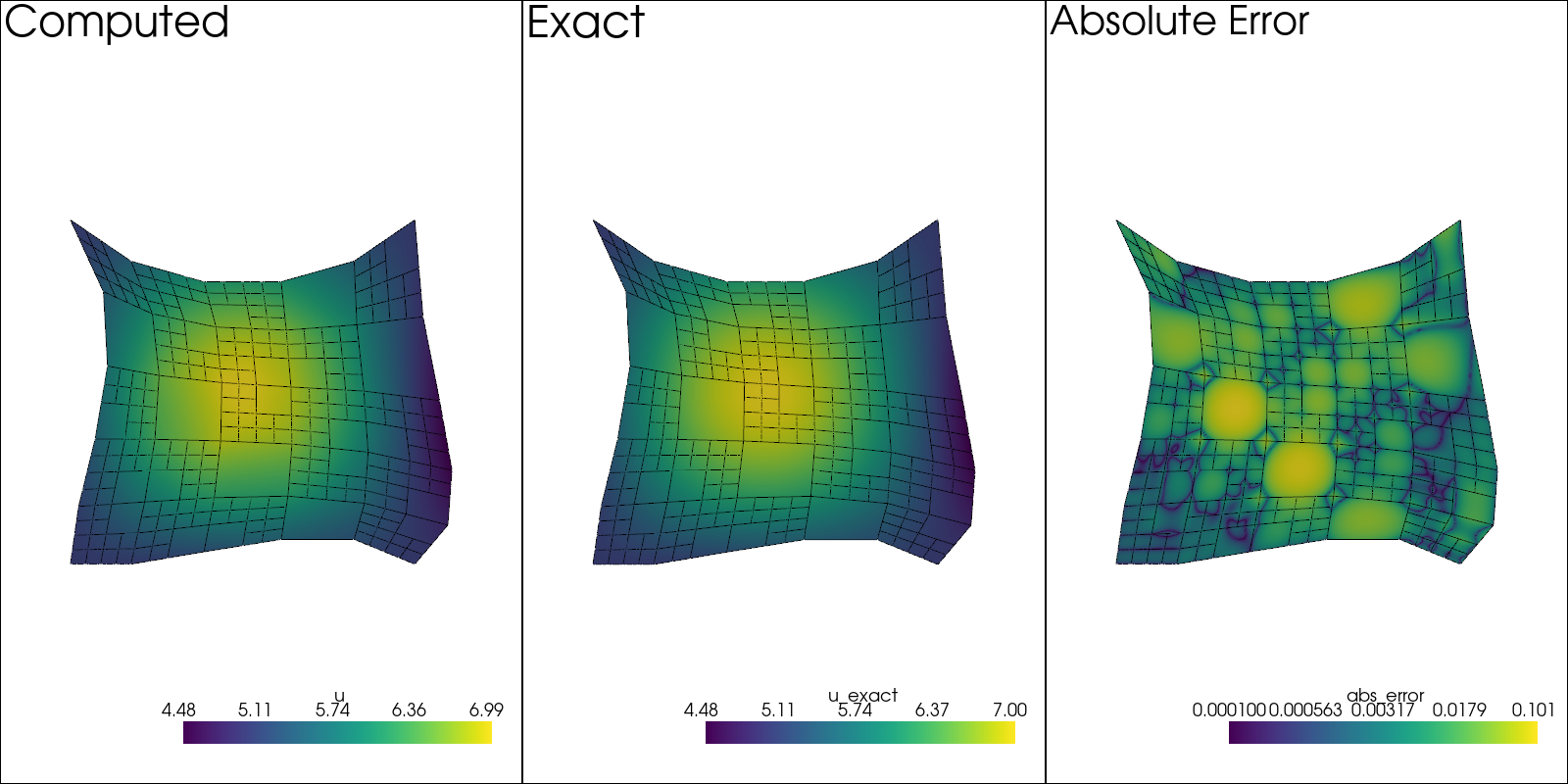
plotter.subplot(0, 0)
plotter.add_mesh(sol.copy(), scalars=u.label, show_scalar_bar=True)
plotter.add_mesh(edges, color="black")
plotter.add_text("Computed")
plotter.view_xy()

sol.point_data["u_exact"] = u_exact(sol.points[:, 0], sol.points[:, 1])
plotter.subplot(0, 1)
plotter.add_mesh(sol.copy(), scalars="u_exact", show_scalar_bar=True)
plotter.add_mesh(edges, color="black")
plotter.add_text("Exact")
plotter.view_xy()

# Error at strong BCs is ~10^{-30}, so make sure to add this
# value, otherwise it will ruin the colormap scale.
sol.point_data["abs_error"] = (
    np.abs(sol.point_data["u_exact"] - sol.point_data[u.label]) + 1e-4
)
plotter.subplot(0, 2)
plotter.add_mesh(sol.copy(), scalars="abs_error", show_scalar_bar=True, log_scale=True)
plotter.add_mesh(edges, color="black")
plotter.add_text("Absolute Error")
plotter.view_xy()

#
# Computing the Results
# ---------------------
#
# Just as was done for the un-refined result, here :math:`L^2` and :math:`H^1` errors
# are computed.
#

p_vals = np.arange(1, 7)
h1_err = np.zeros(p_vals.size)
l2_err = np.zeros(p_vals.size)


for ip, pval in enumerate(p_vals):
    base_mesh = mesh_create(
        pval, np.stack((m.pos_x, m.pos_y), axis=-1), m.lines + 1, m.surfaces
    )

    def refine_test(m: Mesh, i: int):
        """Check if element should be refined."""
        corners = m.get_leaf_corners(i)
        if np.any(np.linalg.norm(corners, axis=-1) > 0.5):
            order = m.get_leaf_orders(i)
            return order, order, order, order
        # Do not refine
        return None

    mesh = base_mesh.split_depth_first(2, refine_test)

    solution, stats, mesh = solve_system_2d(
        mesh,
        system_settings=SystemSettings(
            system,
            boundary_conditions=[
                BoundaryCondition2DSteady(u, mesh.boundary_indices, u_exact)
            ],
        ),
        solver_settings=SolverSettings(absolute_tolerance=1e-10, relative_tolerance=0),
        print_residual=False,
        recon_order=25,
    )

    sol = solution[-1]
    sol.point_data["u_err2"] = (
        sol.point_data["u"] - u_exact(sol.points[:, 0], sol.points[:, 1])
    ) ** 2
    sol.point_data["q_err2"] = np.linalg.norm(
        sol.point_data["q"] - q_exact(sol.points[:, 0], sol.points[:, 1]), axis=-1
    )

    total_error = sol.integrate_data()
    h1_err[ip] = total_error.point_data["q_err2"][0]
    l2_err[ip] = np.sqrt(total_error.point_data["u_err2"][0])
    print(f"Finished {pval=:d}")

Finished pval=1
Finished pval=2
Finished pval=3
Finished pval=4
Finished pval=5
Finished pval=6

Results in \(H^1\) Norm

k1, k0 = np.polyfit((p_vals), np.log(h1_err), 1)
k1, k0 = np.exp(k1), np.exp(k0)

print(f"Solution converges with p as: {k0:.3g} * ({k1:.3g}) ** p in H1")
plt.figure()

plt.scatter(p_vals, h1_err)
plt.semilogy(
    p_vals,
    k0 * k1**p_vals,
    label=f"${k0:.3g} \\cdot \\left( {{{k1:+.3g}}}^p \\right)$",
    linestyle="dashed",
)
plt.gca().set(
    xlabel="$p$",
    ylabel="$\\left|\\left| \\nabla \\ times u - \\nabla \\times \\bar{u}"
    " \\right|\\right|$",
    yscale="log",
)
plt.legend()
plt.grid()
plt.show()

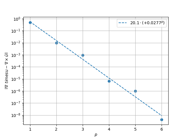
Solution converges with p as: 20.1 * (0.0277) ** p in H1

Results in \(L^2\) Norm

k1, k0 = np.polyfit((p_vals), np.log(l2_err), 1)
k1, k0 = np.exp(k1), np.exp(k0)

print(f"Solution converges with p as: {k0:.3g} * ({k1:.3g}) ** p in L2")
plt.figure()

plt.scatter(p_vals, l2_err)
plt.semilogy(
    p_vals,
    k0 * k1**p_vals,
    label=f"${k0:.3g} \\cdot \\left( {{{k1:+.3g}}}^p \\right)$",
    linestyle="dashed",
)
plt.gca().set(
    xlabel="$p$",
    ylabel="$\\left|\\left| u - \\bar{u} \\right|\\right|$",
    yscale="log",
)
plt.legend()
plt.grid()
plt.show()

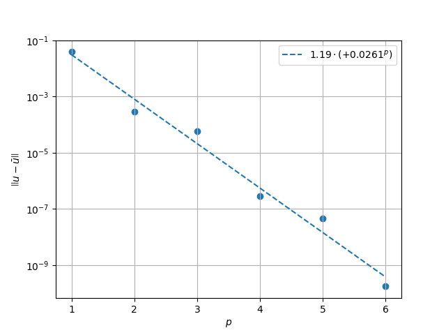
Solution converges with p as: 1.19 * (0.0261) ** p in L2