Poisson Equation in the Direct Formulation

This example shows how the Poisson equation can be solved using the direct formulation. This means that the equation (1) is formulated directly without any intermediate steps.

(1)\[\nabla^2 u = - f\]

The direct formulation requires that the unknown \(u\) be a differential 0-form, defined in \(H(\mathrm{curl})\). As such, the equation to be solved is given by equation (2).

(2)\[\star \mathrm{d} \star \mathrm{d} u^{(0)} = -f^{(0)}\]

This can be rewritten in the variational form as per equation (3)

(3)\[\int_\Omega \mathrm{d} v^{(0)} \wedge \star \mathrm{d} u^{(0)} = \int_\Omega v^{(0)} \wedge \star f^{(0)} + \int_{\partial \Omega} v^{(0)} \wedge \star \mathrm{d} u^{(0)} \quad \forall v^{(0)} \in \Lambda^{(0)}\left( \mathcal{M} \right)\]

Error for this case will be measured in two ways. First is in the typical \(L^2\) norm defined by equation (4).

(4)\[\varepsilon_{L^2}(u) = \sqrt{\int_\Omega \left( u_\mathrm{exact} - u\right) {\mathrm{d}\Omega}}\]

The second is the semi-norm defined by equation (5). The reason to also use this norm, is that is is the norm which is induced by the Laplace operator, which the Poisson equation is defined with.

(5)\[\varepsilon_{H^1}(u) = \int_\Omega \left|\left| \nabla \times u_\mathrm{exact} - \nabla \times u \right|\right| {\mathrm{d}\Omega}\]

import numpy as np
import numpy.typing as npt
import pyvista as pv
import rmsh
from matplotlib import pyplot as plt
from mfv2d import (
    BoundaryCondition2DSteady,
    KFormSystem,
    KFormUnknown,
    Mesh2D,
    SolverSettings,
    SystemSettings,
    UnknownFormOrder,
    solve_system_2d,
)

Setup

The first thing is to setup the necessary prerequisites. This first of all means defining the manufactured solution used for the verification. The manufactured solution for \(u^{(0)}\) is given by equation (6), with its curl \(q^{(1)}\) given by equation (7).

(6)\[u^{(0)}(x, y) = 2 \cos\left(\frac{\pi x}{2}\right) \cos\left(\frac{\pi y}{2}\right)\]

(7)\[q^{(1)}(x, y) = - \pi \cos\left(\frac{\pi x}{2}\right) \sin\left(\frac{\pi y}{2}\right) dx + \pi \sin\left(\frac{\pi x}{2}\right) \cos\left(\frac{\pi y}{2}\right) dy\]

The source term on the right side of the equation is thus given by equation (8).

(8)\[f^{(0)}(x, y) = - \pi^2 \cos\left(\frac{\pi x}{2}\right) \cos\left(\frac{\pi y}{2}\right)\]

def u_exact(x: npt.NDArray[np.float64], y: npt.NDArray[np.float64]):
    """Exact solution."""
    return 2 * np.cos(np.pi / 2 * x) * np.cos(np.pi / 2 * y) + 5


def q_exact(x: npt.NDArray[np.float64], y: npt.NDArray[np.float64]):
    """Exact curl of solution."""
    return np.stack(
        (
            -np.pi * np.cos(np.pi / 2 * x) * np.sin(np.pi / 2 * y),
            np.pi * np.sin(np.pi / 2 * x) * np.cos(np.pi / 2 * y),
        ),
        axis=-1,
    )


def source_exact(x: npt.NDArray[np.floating], y: npt.NDArray[np.floating]):
    """Exact divergence."""
    return -(np.pi**2) * np.cos(np.pi / 2 * x) * np.cos(np.pi / 2 * y)

System Setup

Here the system is set up. An additional unknown \(q^{(1)}\) is introduced. This is just to compute the curl of the solution along with it. The equations in the system bellow are first repeating equation (3), then followed by newly introduced equation (9), which just ensures that \(q^{(1)}\) is equal to the curl of \(u^{(0)}\), since that is needed to compute the error given by the \(H^1\).

(9)\[\int_\Omega p^{(1)} \wedge \star \mathrm{d} u^{(0)} - \int_\Omega p^{(1)} \wedge \star q^{(1)} = 0\]

u = KFormUnknown("u", UnknownFormOrder.FORM_ORDER_0)
v = u.weight
q = KFormUnknown("q", UnknownFormOrder.FORM_ORDER_1)
p = q.weight

system = KFormSystem(
    v.derivative * u.derivative == -(v * source_exact) + (v ^ q_exact),
    p * u.derivative - p * q == 0,
    sorting=lambda f: f.order,
)
print(system)

[u(1*)]^T  ([(E(2, 1))^T @ M(1) @ E(2, 1) |         0]  [u(0)]   [-1 * <u, source_exact> + <u, q_exact>])
[q(2*)]    ([              M(2) @ E(2, 1) | -1 * M(2)]  [q(1)] = [                                    0])

Making The Mesh

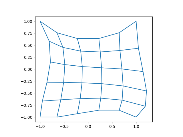
The mesh this is being solved on is a a single block of 6 by 6 quatrilaterals. The boundaries of the mesh are defined by B-splines with 4 knots, meaning they are cubic splines. The mesh is presented in the plot bellow.

N = 6
n1 = N
n2 = N

m, rx, ry = rmsh.create_elliptical_mesh(
    rmsh.MeshBlock(
        None,
        rmsh.BoundaryCurve.from_knots(
            n1, (-1, -1), (-0.5, -1.1), (+0.5, -0.6), (+1, -1)
        ),  # bottom
        rmsh.BoundaryCurve.from_knots(
            n2, (+1, -1), (+1.5, -0.7), (+1, 0.0), (+1, +1)
        ),  # right
        rmsh.BoundaryCurve.from_knots(
            n1, (+1, +1), (0.5, 0.5), (-0.5, 0.5), (-1, +1)
        ),  # top
        rmsh.BoundaryCurve.from_knots(
            n2, (-1, +1), (-0.5, 0.33), (-1, -0.5), (-1, -1)
        ),  # left
    )
)
assert rx < 1e-6 and ry < 1e-6

# Show the mesh for the first time.
fig, ax = plt.subplots(1, 1)
xlim, ylim = m.plot(ax)
ax.set_xlim(1.1 * xlim[0], 1.1 * xlim[1])
ax.set_ylim(1.1 * ylim[0], 1.1 * ylim[1])
ax.set_aspect("equal")
plt.show()

Check the Result

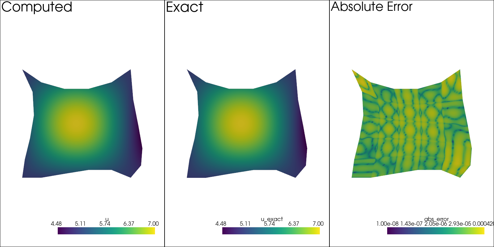
Before checking the convergence, let us first just check on how the solution looks.

pval = 3  # Test polynomial order
msh = Mesh2D(pval, np.stack((m.pos_x, m.pos_y), axis=-1), m.lines + 1, m.surfaces)

solution, stats = solve_system_2d(
    msh,
    system_settings=SystemSettings(
        system,
        boundary_conditions=[BoundaryCondition2DSteady(u, msh.boundary_indices, u_exact)],
    ),
    solver_settings=SolverSettings(absolute_tolerance=1e-10, relative_tolerance=0),
    print_residual=False,
    recon_order=25,
)


sol: pv.UnstructuredGrid = solution[-1]
pv.set_plot_theme("document")
plotter = pv.Plotter(shape=(1, 3), window_size=(1600, 800), off_screen=True)

plotter.subplot(0, 0)
plotter.add_mesh(sol.copy(), scalars=u.label, show_scalar_bar=True)
plotter.add_text("Computed")
plotter.view_xy()

sol.point_data["u_exact"] = u_exact(sol.points[:, 0], sol.points[:, 1])
plotter.subplot(0, 1)
plotter.add_mesh(sol.copy(), scalars="u_exact", show_scalar_bar=True)
plotter.add_text("Exact")
plotter.view_xy()

# Error at strong BCs is ~10^{-30}, so make sure to add this
# value, otherwise it will ruin the colormap scale.
sol.point_data["abs_error"] = (
    np.abs(sol.point_data["u_exact"] - sol.point_data[u.label]) + 1e-8
)
plotter.subplot(0, 2)
plotter.add_mesh(sol.copy(), scalars="abs_error", show_scalar_bar=True, log_scale=True)
plotter.add_text("Absolute Error")
plotter.view_xy()

# plotter.show()

Solve for Different Orders

So we solve for different orders.

p_vals = np.arange(1, 7)
h1_err = np.zeros(p_vals.size)
l2_err = np.zeros(p_vals.size)

for ip, pval in enumerate(p_vals):
    msh = Mesh2D(pval, np.stack((m.pos_x, m.pos_y), axis=-1), m.lines + 1, m.surfaces)

    solution, stats = solve_system_2d(
        msh,
        system_settings=SystemSettings(
            system,
            boundary_conditions=[
                BoundaryCondition2DSteady(u, msh.boundary_indices, u_exact)
            ],
        ),
        solver_settings=SolverSettings(absolute_tolerance=1e-10, relative_tolerance=0),
        print_residual=False,
        recon_order=25,
    )

    sol = solution[-1]
    sol.point_data["q_err2"] = np.linalg.norm(
        sol.point_data["q"] - q_exact(sol.points[:, 0], sol.points[:, 1]), axis=-1
    )
    sol.point_data["u_err2"] = (
        sol.point_data["u"] - u_exact(sol.points[:, 0], sol.points[:, 1])
    ) ** 2

    total_error = sol.integrate_data()
    h1_err[ip] = total_error.point_data["q_err2"][0]
    l2_err[ip] = np.sqrt(total_error.point_data["u_err2"][0])
    print(f"Finished {pval=:d}")

Finished pval=1
Finished pval=2
Finished pval=3
Finished pval=4
Finished pval=5
Finished pval=6

Plot Results

Here we plot the results.

\(H^1\) Norm

k1, k0 = np.polyfit((p_vals), np.log(h1_err), 1)
k1, k0 = np.exp(k1), np.exp(k0)

print(f"Solution converges with p as: {k0:.3g} * ({k1:.3g}) ** p in H1 norm")
plt.figure()

plt.scatter(p_vals, h1_err)
plt.semilogy(
    p_vals,
    k0 * k1**p_vals,
    label=f"${k0:.3g} \\cdot \\left( {{{k1:+.3g}}}^p \\right)$",
    linestyle="dashed",
)
plt.gca().set(
    xlabel="$p$",
    ylabel="$\\left|\\left| \\nabla \\times u - \\nabla \\times"
    " \\bar{u} \\right|\\right|$",
    yscale="log",
)
plt.legend()
plt.grid()
plt.show()

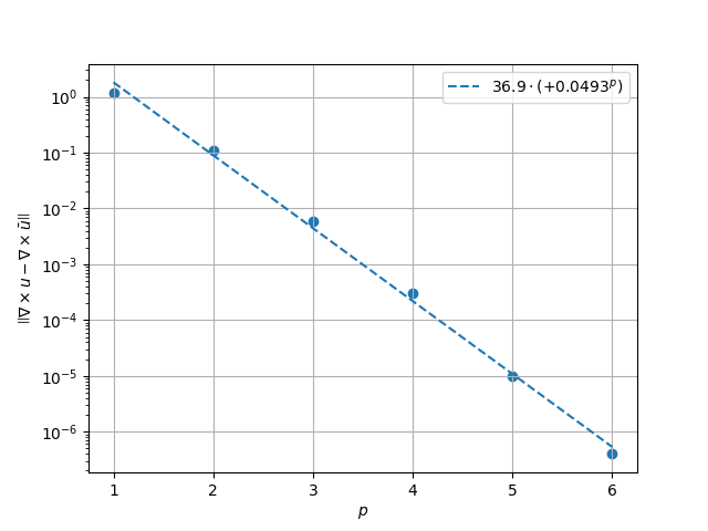
Solution converges with p as: 36.9 * (0.0493) ** p in H1 norm

\(L^2\) Norm

k1, k0 = np.polyfit((p_vals), np.log(l2_err), 1)
k1, k0 = np.exp(k1), np.exp(k0)

print(f"Solution converges with p as: {k0:.3g} * ({k1:.3g}) ** p in L2 norm.")
plt.figure()

plt.scatter(p_vals, l2_err)
plt.semilogy(
    p_vals,
    k0 * k1**p_vals,
    label=f"${k0:.3g} \\cdot \\left( {{{k1:+.3g}}}^p \\right)$",
    linestyle="dashed",
)
plt.gca().set(
    xlabel="$p$",
    ylabel="$\\varepsilon_{L^2}$",
    yscale="log",
)
plt.legend()
plt.grid()
plt.show()

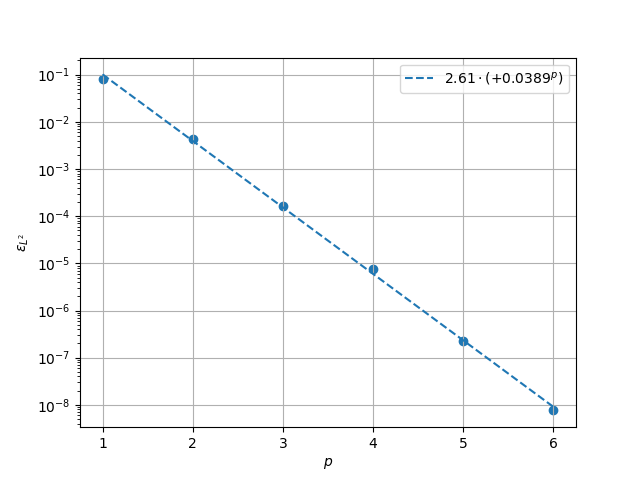
Solution converges with p as: 2.61 * (0.0389) ** p in L2 norm.