Linear Advection-Diffusion

This example shows how linear advection-diffusion equation can be solved. There are of course two main ways:

• direct formulation

• mixed formulation

Both case solve the same equation, given by formulation. This means that the equation (1). With differential geometry it is written as either (2) for the direct formulation or as (3) in the mixed formulation.

(1)\[\begin{split}\vec{a}(x, y) \cdot \nabla u + \nu \nabla^2 u = -f \quad \vec{a} = \begin{bmatrix} a_x(x, y) \\ a_y(x, y) \end{bmatrix}\end{split}\]

(2)\[\begin{split}\mathrm{d} i_{\hat{a}} \mathrm{d} u^{(0)} + \nu \star \mathrm{d} \star \mathrm{d} u^{(0)} = -f^{(0)} \quad \hat{a} = \begin{bmatrix} a_y \\ -a_x \end{bmatrix}\end{split}\]

(3)\[\begin{split}-\star i_{\vec{a}} \mathrm{d} \star u^{(2)} + \nu \mathrm{d} \star \mathrm{d} \star \mathrm{d} u^{(2)} = -f^{(2)} \quad \vec{a} = \begin{bmatrix} a_x(x, y) \\ a_y(x, y) \end{bmatrix}\end{split}\]

The formulation explored here is the mixed formulation given by equation (3). It can also be noted that the problem is quite similar to the mixed Poisson problem, with the only difference being the advective term with the interior product. As such, for anything not explicitly covered here, please refer back to Poisson Equation in the Mixed Formulation.

As with the mixed Poisson, error for this case will be measured in two ways - with the \(L^2\) norm and with the \(H^1\) norm.

import numpy as np
import numpy.typing as npt
import pyvista as pv
import rmsh
from matplotlib import pyplot as plt
from mfv2d import (
    KFormSystem,
    KFormUnknown,
    Mesh2D,
    SolverSettings,
    SystemSettings,
    UnknownFormOrder,
    solve_system_2d,
)

Problem Setup

The problem setup is very similar to the mixed Poisson problem, but now with an addition of the advection vector field, which is given by (4). The presence of the advection term is also changes the source term of the equation.

(4)\[\begin{split}\vec{a} = \begin{bmatrix} 3 y - x \\ 2 - y \end{bmatrix}\end{split}\]

NU = -0.05


def a_field(x: npt.NDArray[np.floating], y: npt.NDArray[np.floating]):
    """Advection vector field."""
    return np.stack(((3 * y - x), (2 - y + 0 * x)), axis=-1)


def u_exact(x: npt.NDArray[np.floating], y: npt.NDArray[np.floating]):
    """Exact solution."""
    return 2 * np.cos(np.pi / 2 * x) * np.cos(np.pi / 2 * y)


def q_exact(x: npt.NDArray[np.floating], y: npt.NDArray[np.floating]):
    """Exact gradient of solution."""
    return np.stack(
        (
            -np.pi * np.sin(np.pi / 2 * x) * np.cos(np.pi / 2 * y),
            -np.pi * np.cos(np.pi / 2 * x) * np.sin(np.pi / 2 * y),
        ),
        axis=-1,
    )


def source_exact(x: npt.NDArray[np.floating], y: npt.NDArray[np.floating]):
    """Exact source term."""
    return (
        np.sum(a_field(x, y) * q_exact(x, y), axis=-1) - NU * np.pi**2 * u_exact(x, y) / 2
    )

System Setup

As expected, the system now has the interior product term added, together with the diffusion coefficient \(\nu\) being added.

u = KFormUnknown("u", UnknownFormOrder.FORM_ORDER_2)
v = u.weight
q = KFormUnknown("q", UnknownFormOrder.FORM_ORDER_1)
p = q.weight

system = KFormSystem(
    p.derivative * u - p * q == p ^ u_exact,
    NU * (v * q.derivative) - (v * (a_field * ~q)) == -(v * source_exact),
    sorting=lambda f: f.order,
)
print(system)

[q(2*)]^T  ([                                                    -1 * M(2) | (E(3, 2))^T @ M(2)]  [q(1)]   [          <q, u_exact>])
[u(3*)]    ([(-0.05 * M(3) @ E(3, 2) - 1 * M(3) @ M(1, 2; a_field) @ M(2)) |                  0]  [u(2)] = [-1 * <u, source_exact>])

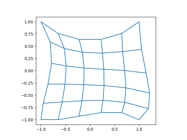
Making the Mesh

The mesh is exactly the same as was the case for the mixed Poisson example.

N = 6
n1 = N
n2 = N

m, rx, ry = rmsh.create_elliptical_mesh(
    rmsh.MeshBlock(
        None,
        rmsh.BoundaryCurve.from_knots(
            n1, (-1, -1), (-0.5, -1.1), (+0.5, -0.6), (+1, -1)
        ),  # bottom
        rmsh.BoundaryCurve.from_knots(
            n2, (+1, -1), (+1.5, -0.7), (+1, 0.0), (+1, +1)
        ),  # right
        rmsh.BoundaryCurve.from_knots(
            n1, (+1, +1), (0.5, 0.5), (-0.5, 0.5), (-1, +1)
        ),  # top
        rmsh.BoundaryCurve.from_knots(
            n2, (-1, +1), (-0.5, 0.33), (-1, -0.5), (-1, -1)
        ),  # left
    )
)
assert rx < 1e-6 and ry < 1e-6
fig, ax = plt.subplots(1, 1)
xlim, ylim = m.plot(ax)
ax.set_xlim(1.1 * xlim[0], 1.1 * xlim[1])
ax.set_ylim(1.1 * ylim[0], 1.1 * ylim[1])
ax.set_aspect("equal")
plt.show()

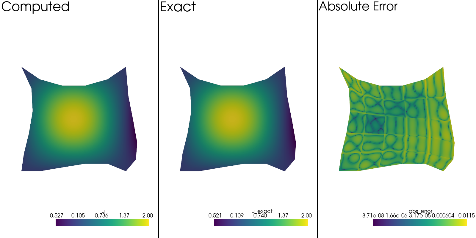
Check the Result

Before checking the convergence, let us first just check on how the solution looks.

pval = 3
msh = Mesh2D(pval, np.stack((m.pos_x, m.pos_y), axis=-1), m.lines + 1, m.surfaces)

solution, stats = solve_system_2d(
    msh,
    system_settings=SystemSettings(system),
    solver_settings=SolverSettings(absolute_tolerance=1e-10, relative_tolerance=0),
    print_residual=False,
    recon_order=25,
)


sol: pv.UnstructuredGrid = solution[-1]
pv.set_plot_theme("document")
plotter = pv.Plotter(shape=(1, 3), window_size=(1600, 800), off_screen=True)

plotter.subplot(0, 0)
plotter.add_mesh(sol.copy(), scalars=u.label, show_scalar_bar=True)
plotter.add_text("Computed")
plotter.view_xy()

sol.point_data["u_exact"] = u_exact(sol.points[:, 0], sol.points[:, 1])
plotter.subplot(0, 1)
plotter.add_mesh(sol.copy(), scalars="u_exact", show_scalar_bar=True)
plotter.add_text("Exact")
plotter.view_xy()

sol.point_data["abs_error"] = np.abs(sol.point_data["u_exact"] - sol.point_data[u.label])
plotter.subplot(0, 2)
plotter.add_mesh(sol.copy(), scalars="abs_error", show_scalar_bar=True, log_scale=True)
plotter.add_text("Absolute Error")
plotter.view_xy()

Solve for Different Orders

So we solve for different orders.

p_vals = np.arange(1, 7)
h1_err = np.zeros(p_vals.size)
l2_err = np.zeros(p_vals.size)

for ip, pval in enumerate(p_vals):
    msh = Mesh2D(pval, np.stack((m.pos_x, m.pos_y), axis=-1), m.lines + 1, m.surfaces)

    solution, stats = solve_system_2d(
        msh,
        system_settings=SystemSettings(system),
        solver_settings=SolverSettings(absolute_tolerance=1e-10, relative_tolerance=0),
        print_residual=False,
        recon_order=25,
    )

    sol = solution[-1]

    sol.point_data["q_err2"] = np.linalg.norm(
        sol.point_data["q"] - q_exact(sol.points[:, 0], sol.points[:, 1]), axis=-1
    )
    sol.point_data["u_err2"] = (
        sol.point_data["u"] - u_exact(sol.points[:, 0], sol.points[:, 1])
    ) ** 2

    total_error = sol.integrate_data()
    h1_err[ip] = total_error.point_data["q_err2"][0]
    l2_err[ip] = np.sqrt(total_error.point_data["u_err2"])[0]
    print(f"Finished {pval=:d}")

Finished pval=1
Finished pval=2
Finished pval=3
Finished pval=4
Finished pval=5
Finished pval=6

Plot Results

Here we plot the results.

\(H^1\) Norm

k1, k0 = np.polyfit((p_vals), np.log(h1_err), 1)
k1, k0 = np.exp(k1), np.exp(k0)

print(f"Solution converges with p as: {k0:.3g} * ({k1:.3g}) ** p in H1 norm")
plt.figure()

plt.scatter(p_vals, h1_err)
plt.semilogy(
    p_vals,
    k0 * k1**p_vals,
    label=f"${k0:.3g} \\cdot \\left( {{{k1:+.3g}}}^p \\right)$",
    linestyle="dashed",
)
plt.gca().set(
    xlabel="$p$",
    ylabel="$\\int\\left|\\left| q - \\bar{q} \\right|\\right|$",
    yscale="log",
)
plt.legend()
plt.grid()
plt.show()

Solution converges with p as: 32.6 * (0.0472) ** p in H1 norm

\(L^2\) Norm

k1, k0 = np.polyfit((p_vals), np.log(l2_err), 1)
k1, k0 = np.exp(k1), np.exp(k0)

print(f"Solution converges with p as: {k0:.3g} * ({k1:.3g}) ** p in L2 norm.")
plt.figure()

plt.scatter(p_vals, l2_err)
plt.semilogy(
    p_vals,
    k0 * k1**p_vals,
    label=f"${k0:.3g} \\cdot \\left( {{{k1:+.3g}}}^p \\right)$",
    linestyle="dashed",
)
plt.gca().set(
    xlabel="$p$",
    ylabel="$\\varepsilon_{L^2}$",
    yscale="log",
)
plt.legend()
plt.grid()
plt.show()

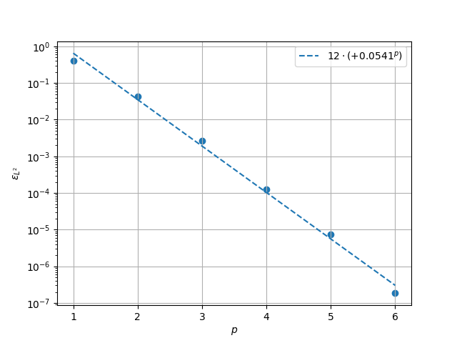
Solution converges with p as: 12 * (0.0541) ** p in L2 norm.