Stokes Flow

Stokes flow is a steady state solution to the Poisson equation, with an added incompressibility constraint. It is also the symmetric part of Navier-Stokes equations, so solving it is the first step in solving Navier-Stokes.

The full system is given by (1).

(1)\[\omega - \nabla \times u = 0 -\nabla \omega + \nabla p = f \nabla \cdot u = 0\]

When written with differential geometry, it becomes system (2). This can be written in the variational form as system (3).

(2)\[ \begin{align}\begin{aligned}\omega^{(0)} - \star \mathrm{d} \star u^{(1)} = 0\\-\mathrm{d} \omega^{(0)} + \star \mathrm{d} \star p^{(2)} = f^{(1)}\\\mathrm{d} u^{(1)} = 0\end{aligned}\end{align} \]

(3)\[ \begin{align}\begin{aligned}\left(\phi^{(0)}, \omega^{(0)}\right)_\Omega - \left(\mathrm{d} p^{(0)}, u^{(1)}\right)_\Omega = \int_{\partial \Omega} \phi^{(0)} \wedge \star u^{(1)}\quad\forall \phi^{(0)} \in \Lambda^{(0)}(\mathcal{M})\\-\left(v^{(1)}, \mathrm{d} \omega^{(0)}\right)_\Omega + \left(\mathrm{d} v^{(1)}, p^{(2)}\right)_\Omega = \left(v^{(1)}, f^{(1)}\right)_\Omega + \int_{\partial \Omega} v^{(1)} \wedge \star p^{(2)}\quad\forall v^{(1)} \in \Lambda^{(1)}(\mathcal{M})\\\left(r^{(2)}, \mathrm{d} u^{(1)}\right)_\Omega = 0 \quad\forall r^{(2)} \in \Lambda^{(2)}(\mathcal{M})\end{aligned}\end{align} \]

import numpy as np
import numpy.typing as npt
import pyvista as pv
import rmsh
from matplotlib import pyplot as plt
from mfv2d import (
    BoundaryCondition2DSteady,
    KFormSystem,
    KFormUnknown,
    Mesh2D,
    SolverSettings,
    SystemSettings,
    UnknownFormOrder,
    solve_system_2d,
)

Setup

The manufactured solution for this case is the velocity field given by (4), which gives the exact vorticity as per (5). As for the pressure, it is given by FUCKING BLACK MAGIC, I HAVE NO CLUE WHY THE FUCK IT IS NON-ZERO! IS THIS SOME SORT OF A FUCKING CRUEL JOKE, GOD?

(4)\[u^{(1)}(x, y) = \sin(x) \cos(y) dy - (- \cos(x) \sin(y)) dx\]

(5)\[\omega^{(0)}(x, y) = - 2 \sin(x) \sin(y)\]

This together gives the momentum source as per (6).

(6)\[f^{(1)} = -2 (\sin(x) \cos(y) dy - (-\cos(x) \sin(y)) dx)\]

def vel_exact(x: npt.NDArray[np.float64], y: npt.NDArray[np.float64]):
    """Exact velocity."""
    return np.stack(
        (np.sin(x) * np.cos(y), -np.cos(x) * np.sin(y)),
        axis=-1,
    )


# TODO: ???
def prs_exact(x, y):
    """Exact pressure."""
    return 0 * x * y


def vor_exact(x, y):
    """Exact vorticity."""
    return -2 * np.sin(x) * np.sin(y) + 0 * x * y


def momentum_source(x, y):
    """Exact momentum equation source term."""
    return -2 * np.stack((np.sin(x) * np.cos(y), -np.cos(x) * np.sin(y)), axis=-1)

System Setup

The system is setup in the same way as described in (3). Additionally, boundary conditions will be applied for velocity both strongly (for normal velocity) and weakly (for the tangential velocity).

One tweak made here is the inclusion of the div unknown, which is just equated to the divergence of \(u^{(1)}\). The reason for this is the demonstration in the later section of how the divergence behaves.

prs = KFormUnknown("prs", UnknownFormOrder.FORM_ORDER_2)
w_prs = prs.weight
vel = KFormUnknown("vel", UnknownFormOrder.FORM_ORDER_1)
w_vel = vel.weight
vor = KFormUnknown("vor", UnknownFormOrder.FORM_ORDER_0)
w_vor = vor.weight
div = KFormUnknown("div", UnknownFormOrder.FORM_ORDER_2)
w_div = div.weight

system = KFormSystem(
    w_vor.derivative * vel + w_vor * vor == w_vor ^ vel_exact,
    w_vel * vor.derivative + w_vel.derivative * prs
    == (w_vel ^ prs_exact) + w_vel * momentum_source,
    w_prs * vel.derivative == 0,
    w_div * div - w_div * vel.derivative == 0,
    sorting=lambda f: f.order,
)
print(system)

[vor(1*)]^T  ([          M(1) |  (E(2, 1))^T @ M(1) |                  0 |    0]  [vor(0)]   [                         <vor, vel_exact>])
[vel(2*)]    ([M(2) @ E(2, 1) |                   0 | (E(3, 2))^T @ M(2) |    0]  [vel(1)]   [<vel, prs_exact> + <vel, momentum_source>])
[prs(3*)]    ([             0 |      M(3) @ E(3, 2) |                  0 |    0]  [prs(2)] = [                                        0])
[div(3*)]    ([             0 | -1 * M(3) @ E(3, 2) |                  0 | M(3)]  [div(2)]   [                                        0])

Making the Mesh

The mesh is the same mess as for all the other examples of steady problems.

N = 6
n1 = N
n2 = N
m, rx, ry = rmsh.create_elliptical_mesh(
    rmsh.MeshBlock(
        None,
        rmsh.BoundaryCurve.from_knots(
            n1, (-1, -1), (-0.5, -1.1), (+0.5, -0.6), (+1, -1)
        ),  # bottom
        rmsh.BoundaryCurve.from_knots(
            n2, (+1, -1), (+1.5, -0.7), (+1, 0.0), (+1, +1)
        ),  # right
        rmsh.BoundaryCurve.from_knots(
            n1, (+1, +1), (0.5, 0.5), (-0.5, 0.5), (-1, +1)
        ),  # top
        rmsh.BoundaryCurve.from_knots(
            n2, (-1, +1), (-0.5, 0.33), (-1, -0.5), (-1, -1)
        ),  # left
    )
)
assert rx < 1e-6 and ry < 1e-6
fig, ax = plt.subplots(1, 1)
xlim, ylim = m.plot(ax)
ax.set_xlim(1.1 * xlim[0], 1.1 * xlim[1])
ax.set_ylim(1.1 * ylim[0], 1.1 * ylim[1])
ax.set_aspect("equal")
plt.show()

Check the Results

One important property of MSEM is that the way it is formulated allows for exact strong derivatives. The consequence of that is that the incompressibility constraint given by equation (7) is enforced exactly. Whatever solution is obtained is divergence free down to machine precision.

(7)\[\left(r^{(2)}, d u^{(1)} \right)_\Omega = 0 \quad r^{(2)} \in \Lambda^{(2)}(\mathcal(M))\]

pval = 3
msh = Mesh2D(pval, np.stack((m.pos_x, m.pos_y), axis=-1), m.lines + 1, m.surfaces)

solution, stats = solve_system_2d(
    msh,
    system_settings=SystemSettings(
        system,
        constrained_forms=[(0.0, prs)],
        boundary_conditions=[
            BoundaryCondition2DSteady(vel, msh.boundary_indices, vel_exact)
        ],
    ),
    solver_settings=SolverSettings(
        absolute_tolerance=1e-10, relative_tolerance=0, maximum_iterations=1
    ),
    recon_order=25,
)

sol: pv.UnstructuredGrid = solution[-1]


plotter = pv.Plotter(off_screen=True, shape=(1, 1), window_size=(1600, 800))

sol.point_data["div"] = np.abs(sol.point_data["div"])
plotter.add_mesh(sol, scalars="div", log_scale=True, show_scalar_bar=True)
plotter.add_mesh(sol.extract_all_edges(), color="black")
plotter.view_xy()
print(f"Highest value of divergence in the domain is {sol.point_data['div'].max():.3e}")

Highest value of divergence in the domain is 9.183e-15

Solve for Different Orders

So we solve for different orders. Before that, we remake the system without the divergence form.

system = KFormSystem(
    w_vor.derivative * vel + w_vor * vor == w_vor ^ vel_exact,
    w_vel * vor.derivative + w_vel.derivative * prs
    == (w_vel ^ prs_exact) + w_vel * momentum_source,
    w_prs * vel.derivative == 0,
    sorting=lambda f: f.order,
)

p_vals = np.arange(1, 7)
h1_err = np.zeros(p_vals.size)
l2_err = np.zeros(p_vals.size)

for ip, pval in enumerate(p_vals):
    msh = Mesh2D(pval, np.stack((m.pos_x, m.pos_y), axis=-1), m.lines + 1, m.surfaces)

    solution, stats = solve_system_2d(
        msh,
        system_settings=SystemSettings(
            system,
            constrained_forms=[(0.0, prs)],
            boundary_conditions=[
                BoundaryCondition2DSteady(vel, msh.boundary_indices, vel_exact)
            ],
        ),
        solver_settings=SolverSettings(
            absolute_tolerance=1e-10, relative_tolerance=0, maximum_iterations=1
        ),
        recon_order=25,
    )

    sol = solution[-1]
    sol.point_data["vel_err2"] = np.linalg.norm(
        sol.point_data["vel"] - vel_exact(sol.points[:, 0], sol.points[:, 1]), axis=-1
    )
    sol.point_data["vor_err2"] = sol.point_data["vor"] - vor_exact(
        sol.points[:, 0], sol.points[:, 1]
    )
    sol.point_data["prs_err2"] = np.abs(
        sol.point_data["prs"] - prs_exact(sol.points[:, 0], sol.points[:, 1])
    )

    total_error = sol.integrate_data()

    l2_err[ip] = total_error.point_data["vel_err2"][0]
    h1_err[ip] = np.abs(total_error.point_data["vor_err2"][0])
    print(f"Finished {pval=:d}")

Finished pval=1
Finished pval=2
Finished pval=3
Finished pval=4
Finished pval=5
Finished pval=6

Plot Results

Here we plot the results.

\(H^1\) Norm

The vorticity error.

k1, k0 = np.polyfit((p_vals), np.log(h1_err), 1)
k1, k0 = np.exp(k1), np.exp(k0)

print(f"Solution converges with p as: {k0:.3g} * ({k1:.3g}) ** p in H1 norm.")
plt.figure()

plt.scatter(p_vals, h1_err)
plt.semilogy(
    p_vals,
    k0 * k1**p_vals,
    label=f"${k0:.3g} \\cdot \\left( {{{k1:+.3g}}}^p \\right)$",
    linestyle="dashed",
)
plt.gca().set(
    xlabel="$p$",
    ylabel="$\\left|\\left| \\vec{\\omega} - \\bar{\\omega} \\right|\\right|$",
    yscale="log",
)
plt.legend()
plt.grid()
plt.show()

Solution converges with p as: 0.00146 * (0.0726) ** p in H1 norm.

\(L^2\) Norm

The velocity error.

k1, k0 = np.polyfit((p_vals), np.log(l2_err), 1)
k1, k0 = np.exp(k1), np.exp(k0)

print(f"Solution converges with p as: {k0:.3g} * ({k1:.3g}) ** p in L2 norm.")
plt.figure()

plt.scatter(p_vals, l2_err)
plt.semilogy(
    p_vals,
    k0 * k1**p_vals,
    label=f"${k0:.3g} \\cdot \\left( {{{k1:+.3g}}}^p \\right)$",
    linestyle="dashed",
)
plt.gca().set(
    xlabel="$p$",
    ylabel="$\\varepsilon_{L^2}$",
    yscale="log",
)
plt.legend()
plt.grid()
plt.show()

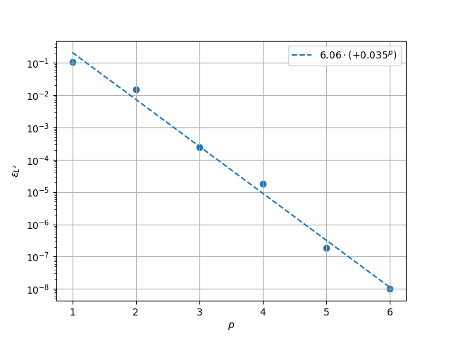
Solution converges with p as: 6.06 * (0.035) ** p in L2 norm.