Poisson Equation with Local Refinement

One of key features of mfv2d is the ability to locally refine the mesh with both hierarchical refinement (divide elements) or with polynomial refinement (increase order of elements).

This examples is otherwise identical to Poisson Equation in the Direct Formulation, where the direct Poisson is solved in a straight-forward manner. As such, only text and comments added to the code are pertaining to features not used in that one.

import numpy as np
import numpy.typing as npt
import pyvista as pv
import rmsh
from matplotlib import pyplot as plt
from mfv2d import (
    BoundaryCondition2DSteady,
    KFormSystem,
    KFormUnknown,
    Mesh2D,
    RefinementSettings,
    SolverSettings,
    SystemSettings,
    UnknownFormOrder,
    solve_system_2d,
)


def u_exact(x: npt.NDArray[np.float64], y: npt.NDArray[np.float64]):
    """Exact solution."""
    return 2 * np.cos(np.pi / 2 * x) * np.cos(np.pi / 2 * y) + 5


def q_exact(x: npt.NDArray[np.float64], y: npt.NDArray[np.float64]):
    """Exact curl of solution."""
    return np.stack(
        (
            -np.pi * np.cos(np.pi / 2 * x) * np.sin(np.pi / 2 * y),
            np.pi * np.sin(np.pi / 2 * x) * np.cos(np.pi / 2 * y),
        ),
        axis=-1,
    )


def source_exact(x: npt.NDArray[np.floating], y: npt.NDArray[np.floating]):
    """Exact heat flux divergence."""
    return -(np.pi**2) * np.cos(np.pi / 2 * x) * np.cos(np.pi / 2 * y)


q = KFormUnknown("q", UnknownFormOrder.FORM_ORDER_1)
p = q.weight
u = KFormUnknown("u", UnknownFormOrder.FORM_ORDER_0)
v = u.weight

system = KFormSystem(
    v.derivative * u.derivative == -(v * source_exact) + (v ^ q_exact),
    p * u.derivative - p * q == 0,
    sorting=lambda f: f.order,
)
print(system)

N = 6
n1 = N
n2 = N


m, rx, ry = rmsh.create_elliptical_mesh(
    rmsh.MeshBlock(
        None,
        rmsh.BoundaryCurve.from_knots(
            n1, (-1, -1), (-0.5, -1.1), (+0.5, -0.6), (+1, -1)
        ),  # bottom
        rmsh.BoundaryCurve.from_knots(
            n2, (+1, -1), (+1.5, -0.7), (+1, 0.0), (+1, +1)
        ),  # right
        rmsh.BoundaryCurve.from_knots(
            n1, (+1, +1), (0.5, 0.5), (-0.5, 0.5), (-1, +1)
        ),  # top
        rmsh.BoundaryCurve.from_knots(
            n2, (-1, +1), (-0.5, 0.33), (-1, -0.5), (-1, -1)
        ),  # left
    )
)
assert rx < 1e-6 and ry < 1e-6

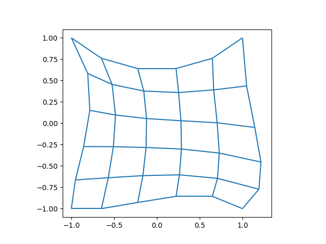
# Show the mesh for the first time.
fig, ax = plt.subplots(1, 1)
xlim, ylim = m.plot(ax)
ax.set_xlim(1.1 * xlim[0], 1.1 * xlim[1])
ax.set_ylim(1.1 * ylim[0], 1.1 * ylim[1])
ax.set_aspect("equal")
plt.show()

pval = 1  # Test polynomial order
msh = Mesh2D(pval, np.stack((m.pos_x, m.pos_y), axis=-1), m.lines + 1, m.surfaces)

[u(1*)]^T  ([(E(2, 1))^T @ M(1) @ E(2, 1) |         0]  [u(0)]   [-1 * <u, source_exact> + <u, q_exact>])
[q(2*)]    ([              M(2) @ E(2, 1) | -1 * M(2)]  [q(1)] = [                                    0])

Refinement Settings

How refinement is done is specified through mfv2d.RefinementSettings. For this example, first the number of division layers is specified. This means that each element and its children can not be divided more than that number of times. The second is the division_predicate, which is called for each element to determine if it should be divided. In this case, it is done quite arbitrarely, being done for every three out of four elements, but it can also use element information to determine whether or not it should occurr.

counter = 0


def division_predicate(_, _idx: int) -> bool:
    """Check if element should be divided."""
    global counter
    cnt = counter
    counter += 1
    return (cnt & 3) != 0


refinement_settings = RefinementSettings(
    refinement_levels=2,
    division_predicate=division_predicate,
)


solution, stats = solve_system_2d(
    msh,
    system_settings=SystemSettings(
        system,
        boundary_conditions=[BoundaryCondition2DSteady(u, msh.boundary_indices, u_exact)],
    ),
    solver_settings=SolverSettings(absolute_tolerance=1e-10, relative_tolerance=0),
    refinement_settings=refinement_settings,
    print_residual=False,
    recon_order=25,
)


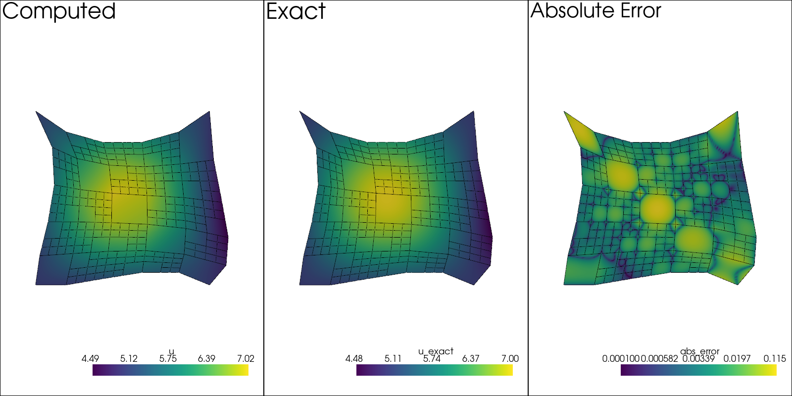
sol: pv.UnstructuredGrid = solution[-1]
pv.set_plot_theme("document")
plotter = pv.Plotter(shape=(1, 3), window_size=(1600, 800), off_screen=True)

edges = sol.extract_all_edges()
plotter.subplot(0, 0)
plotter.add_mesh(sol.copy(), scalars=u.label, show_scalar_bar=True)
plotter.add_mesh(edges, color="black")
plotter.add_text("Computed")
plotter.view_xy()

sol.point_data["u_exact"] = u_exact(sol.points[:, 0], sol.points[:, 1])
plotter.subplot(0, 1)
plotter.add_mesh(sol.copy(), scalars="u_exact", show_scalar_bar=True)
plotter.add_mesh(edges, color="black")
plotter.add_text("Exact")
plotter.view_xy()

# Error at strong BCs is ~10^{-30}, so make sure to add this
# value, otherwise it will ruin the colormap scale.
sol.point_data["abs_error"] = (
    np.abs(sol.point_data["u_exact"] - sol.point_data[u.label]) + 1e-4
)
plotter.subplot(0, 2)
plotter.add_mesh(sol.copy(), scalars="abs_error", show_scalar_bar=True, log_scale=True)
plotter.add_mesh(edges, color="black")
plotter.add_text("Absolute Error")
plotter.view_xy()

#
# Computing the Results
# ---------------------
#
# Just as was done for the un-refined result, here :math:`L^2` and :math:`H^1` errors
# are computed.
#

p_vals = np.arange(1, 7)
h1_err = np.zeros(p_vals.size)
l2_err = np.zeros(p_vals.size)


for ip, pval in enumerate(p_vals):
    msh = Mesh2D(pval, np.stack((m.pos_x, m.pos_y), axis=-1), m.lines + 1, m.surfaces)

    def refine_test(e, i: int) -> bool:
        """Check if element should be refined."""
        del i
        corners = np.array([e.bottom_left, e.bottom_right, e.top_right, e.top_left])
        return bool(np.any(np.linalg.norm(corners, axis=-1) > 0.5))

    def divide_new(
        order: int, level: int, max_level: int
    ) -> tuple[int | None, tuple[int, int, int, int]]:
        """Keep child order equal to parent and set parent to double the child."""
        del level, max_level
        v = order
        return None, (v, v, v, v)

    solution, stats = solve_system_2d(
        msh,
        system_settings=SystemSettings(
            system,
            boundary_conditions=[
                BoundaryCondition2DSteady(u, msh.boundary_indices, u_exact)
            ],
        ),
        solver_settings=SolverSettings(absolute_tolerance=1e-10, relative_tolerance=0),
        refinement_settings=refinement_settings,
        print_residual=False,
        recon_order=25,
    )

    sol = solution[-1]
    sol.point_data["u_err2"] = (
        sol.point_data["u"] - u_exact(sol.points[:, 0], sol.points[:, 1])
    ) ** 2
    sol.point_data["q_err2"] = np.linalg.norm(
        sol.point_data["q"] - q_exact(sol.points[:, 0], sol.points[:, 1]), axis=-1
    )

    total_error = sol.integrate_data()
    h1_err[ip] = total_error.point_data["q_err2"][0]
    l2_err[ip] = np.sqrt(total_error.point_data["u_err2"][0])
    print(f"Finished {pval=:d}")

Finished pval=1
Finished pval=2
Finished pval=3
Finished pval=4
Finished pval=5
Finished pval=6

Results in \(H^1\) Norm

k1, k0 = np.polyfit((p_vals), np.log(h1_err), 1)
k1, k0 = np.exp(k1), np.exp(k0)

print(f"Solution converges with p as: {k0:.3g} * ({k1:.3g}) ** p in H1")
plt.figure()

plt.scatter(p_vals, h1_err)
plt.semilogy(
    p_vals,
    k0 * k1**p_vals,
    label=f"${k0:.3g} \\cdot \\left( {{{k1:+.3g}}}^p \\right)$",
    linestyle="dashed",
)
plt.gca().set(
    xlabel="$p$",
    ylabel="$\\left|\\left| \\nabla \\ times u - \\nabla \\times \\bar{u}"
    " \\right|\\right|$",
    yscale="log",
)
plt.legend()
plt.grid()
plt.show()

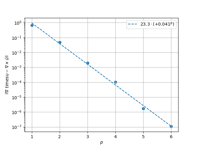
Solution converges with p as: 23.3 * (0.041) ** p in H1

Results in \(L^2\) Norm

k1, k0 = np.polyfit((p_vals), np.log(l2_err), 1)
k1, k0 = np.exp(k1), np.exp(k0)

print(f"Solution converges with p as: {k0:.3g} * ({k1:.3g}) ** p in L2")
plt.figure()

plt.scatter(p_vals, l2_err)
plt.semilogy(
    p_vals,
    k0 * k1**p_vals,
    label=f"${k0:.3g} \\cdot \\left( {{{k1:+.3g}}}^p \\right)$",
    linestyle="dashed",
)
plt.gca().set(
    xlabel="$p$",
    ylabel="$\\left|\\left| u - \\bar{u} \\right|\\right|$",
    yscale="log",
)
plt.legend()
plt.grid()
plt.show()

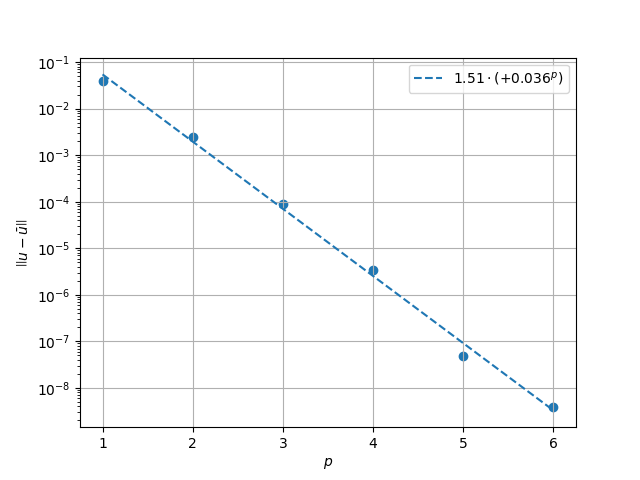
Solution converges with p as: 1.51 * (0.036) ** p in L2