Note
Go to the end to download the full example code.
Incompressible Navier-Stokes Equation#
Incompressible Navier-Stokes is at the heart of modeling low-speed aerodynamics it can be seen as a Stokes flow eqution, with a non-linear source term \(\omega \times u\). The full system is given as per as system (1). When written with differential geometry, it becomes system (2).
The variational form of this system is given by system (3).
import numpy as np
import pyvista as pv
import rmsh
from mfv2d import (
    BoundaryCondition2DSteady,
    ConvergenceSettings,
    KFormSystem,
    KFormUnknown,
    SolverSettings,
    SystemSettings,
    UnknownFormOrder,
    mesh_create,
    solve_system_2d,
    system_as_string,
)
Setup#
The exact solution is given by equation (4). Vorticity is given as per equation (5).
Forcing given for that solution is given by equation (6).
The Reynolds number is also chosen to be \(\mathrm{Re} = 1000\), at which point the advection term is very strongly dominant.
RE = 1e3


def exact_velocty(x, y):
    """Exact velocity solution."""
    return np.stack((np.sin(y) + 0 * x, np.cos(x) + 0 * y), axis=-1)


def exact_vorticity(x, y):
    """Exact vorticity solution."""
    return -(np.sin(x) + np.cos(y))


def exact_forcing(x, y):
    """Exact momentum forcing."""
    return np.stack(
        (
            np.cos(x) * np.cos(y) + 1 / RE * np.sin(y),
            -np.sin(x) * np.sin(y) + 1 / RE * np.cos(x),
        ),
        axis=-1,
    )
System Setup#
The system setup is as can be expected based on the Stokes Flow. The main difference is the addition of the advection term on the right side of the momentum equations.
pre = KFormUnknown("pre", UnknownFormOrder.FORM_ORDER_2)
w_pre = pre.weight
vel = KFormUnknown("vel", UnknownFormOrder.FORM_ORDER_1)
w_vel = vel.weight
vor = KFormUnknown("vor", UnknownFormOrder.FORM_ORDER_0)
w_vor = vor.weight
div = KFormUnknown("div", UnknownFormOrder.FORM_ORDER_2)
w_div = div.weight

system = KFormSystem(
    w_vor.derivative @ vel - w_vor @ vor == w_vor ^ exact_velocty,
    # No weak BC for pressure, since normal velocity is given
    (1 / RE) * (w_vel @ vor.derivative) + w_vel.derivative @ pre
    == w_vel @ exact_forcing - (vel * w_vel @ vor),
    (w_pre @ vel.derivative) == 0,
    w_div @ div - w_div @ vel.derivative == 0,  # Divergence extraction.
)
print(system_as_string(system))
[-1.0 M(0)          | (E(1, 0))^T M(1)  | 0                | 0   ] [vor(0)]   [+ B<vor, exact_velocty>]   [0                     | 0 | 0 | 0] [vor(0)]
[0.001 M(1) E(1, 0) | 0                 | (E(2, 1))^T M(2) | 0   ] [vel(1)]   [+ E<vel, exact_forcing>]   [-1.0 (P(0, 1, vel))^T | 0 | 0 | 0] [vel(1)]
[0                  | M(2) E(2, 1)      | 0                | 0   ] [pre(2)] = [+ 0                    ] + [0                     | 0 | 0 | 0] [pre(2)]
[0                  | -1.0 M(2) E(2, 1) | 0                | M(2)] [div(2)]   [+ 0                    ]   [0                     | 0 | 0 | 0] [div(2)]
Make the Mesh#
The mesh for this problem has to be either fine enough or have high enough elements. Since the problem is non-linear with no initial guess, it can be a bit unstable to compute when under-resolved.
N = 8
P = 6

n1 = N
n2 = N

rect_mesh, rx, ry = rmsh.create_elliptical_mesh(
    rmsh.MeshBlock(
        label=None,
        bottom=rmsh.BoundaryCurve.from_knots(n1, (-1, -1), (+1, -1)),
        right=rmsh.BoundaryCurve.from_knots(n2, (+1, -1), (+1, +1)),
        top=rmsh.BoundaryCurve.from_knots(n1, (+1, +1), (-1, +1)),
        left=rmsh.BoundaryCurve.from_knots(n2, (-1, +1), (-1, -1)),
    )
)
assert rx < 1e-6, ry < 1e-6

mesh = mesh_create(
    P,
    np.stack((rect_mesh.pos_x, rect_mesh.pos_y), axis=-1),
    rect_mesh.lines + 1,
    rect_mesh.surfaces,
)
Solve the System#
Here we solve the system.
solutions, stats, mesh = solve_system_2d(
    mesh,
    SystemSettings(
        system,
        [BoundaryCondition2DSteady(vel, mesh.boundary_indices, exact_velocty)],
        [(0.0, pre)],
    ),
    solver_settings=SolverSettings(
        ConvergenceSettings(
            maximum_iterations=20,
            absolute_tolerance=1e-10,
            relative_tolerance=0,
        )
    ),
    print_residual=False,
    recon_order=25,
)
print(stats)
SolutionStatistics(element_orders={(6, 6): 49}, n_total_dofs=11270, n_leaf_dofs=np.int64(10045), n_lagrange=1225, n_elems=49, n_leaves=49, iter_history=array([2], dtype=uint32), residual_history=array([0.06963362, 0.09025803]))
Print Statistics#
Quick statistics for this solution, such as velocity and vorticity erros are extracted from there.
solution = solutions[-1]

vel_exact = exact_velocty(solution.points[:, 0], solution.points[:, 1])
vor_exact = exact_vorticity(solution.points[:, 0], solution.points[:, 1])

solution.point_data["vel_exact"] = vel_exact
solution.point_data["vor_exact"] = vor_exact

solution.point_data["vel_err"] = np.linalg.norm(
    vel_exact - solution.point_data[vel.label], axis=-1
)
solution.point_data["vor_err"] = np.abs(vor_exact - solution.point_data[vor.label])

integraded = solution.integrate_data()

err_vel = float(integraded.point_data["vel_err"][0])
err_vor = float(integraded.point_data["vor_err"][0])
total_pre = float(integraded.point_data[pre.label][0])

print(f"Integrated pressure is {total_pre:.3e}")
print(f"{err_vel=:.3e}")
print(f"{err_vor=:.3e}")
Integrated pressure is 1.427e-12
err_vel=8.555e-10
err_vor=1.511e-10
Check the Divergence#
As was shown in the Stokes flow example, here the flow is completely divergence flow. This guarantees that the pressure solution is sensible.
plotter = pv.Plotter(off_screen=True, shape=(1, 1), window_size=(1600, 800))

solution.point_data["div"] = np.abs(solution.point_data["div"])
plotter.add_mesh(solution, scalars="div", log_scale=True, show_scalar_bar=True)
plotter.add_mesh(solution.extract_all_edges(), color="black")
plotter.view_xy()
print(
    f"Highest value of divergence in the domain is {solution.point_data['div'].max():.3e}"
)
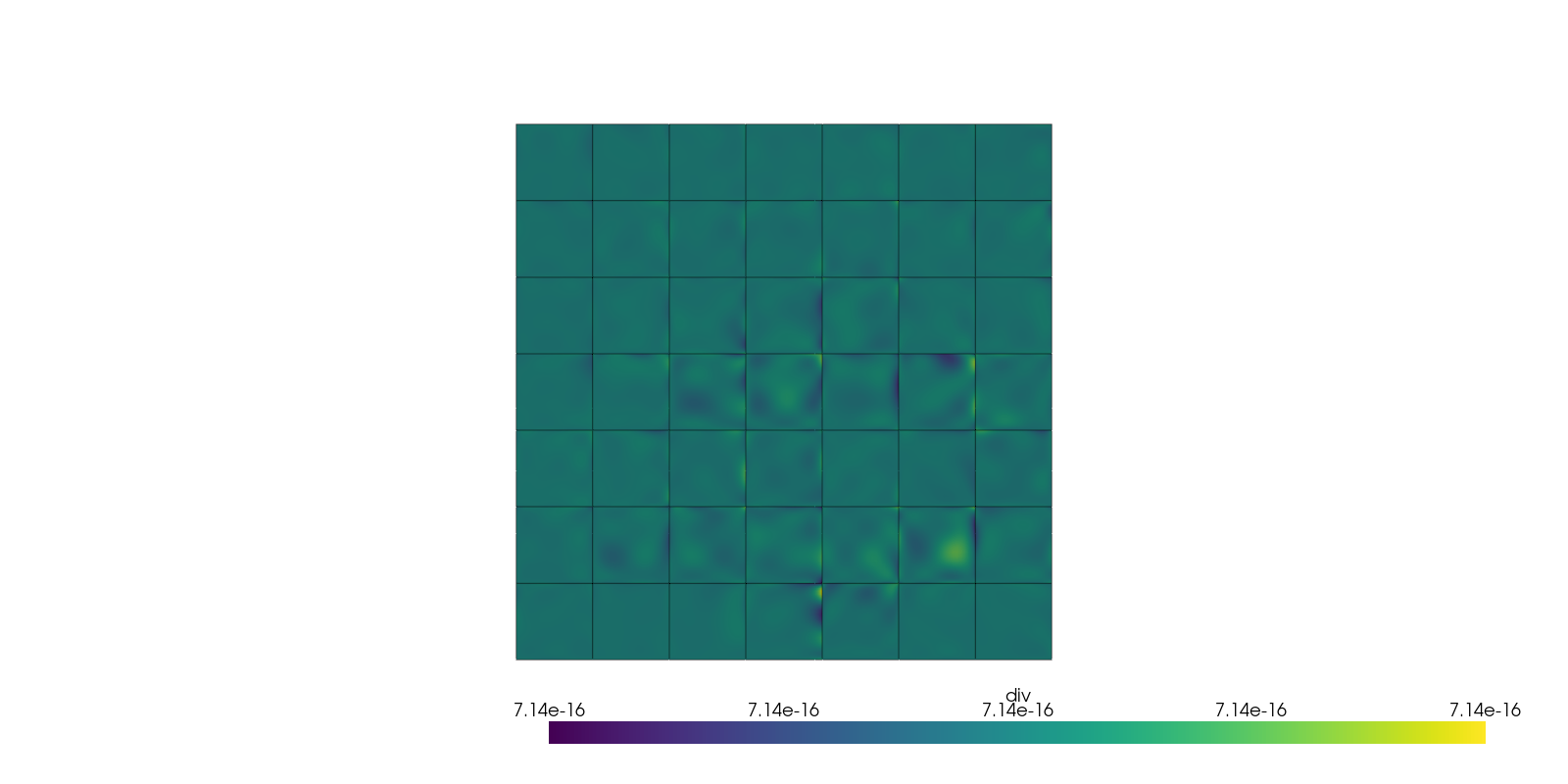
Highest value of divergence in the domain is 2.762e-15
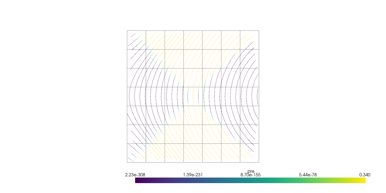
Plot Streamlines#
Pyvista allows for very simple 2D streamline plots.
plotter = pv.Plotter(off_screen=True, shape=(1, 1), window_size=(1600, 800))

solution.point_data["div"] = np.abs(solution.point_data["div"])
solution.point_data["vel"] = np.pad(solution.point_data["vel"], ((0, 0), (0, 1)))
plotter.add_mesh(solution.extract_all_edges(), color="black")
plotter.add_mesh(
    solution.streamlines_evenly_spaced_2D(
        vectors="vel",
        step_length=0.3,
        start_position=(0, 0, 0),
        separating_distance=0.2,
        separating_distance_ratio=0.1,
        compute_vorticity=False,
    ),
    scalars="pre",
    log_scale=True,
    show_scalar_bar=True,
)
plotter.view_xy()
Total running time of the script: (0 minutes 11.259 seconds)