Reaction Equation

The reaction equation is probably the simples non-trivial unsteady differenital equation. It is given by equation (1). If the forcing \(f\) is only space dependent, then it has a very simple analytical solution given by (2), where \(u_\mathrm{initial} = u(x, y, 0)\) and \(u_\mathrm{final} = f(x, y) / \alpha\).

(1)\[\frac{\partial u}{\partial t} + \alpha u = + f\]

(2)\[u(x, y, t) = u_\mathrm{initial} (1 - e^{-\alpha t}) + u_\mathrm{final} e^{-\alpha t}\]

In the 2D case with differential geometry, this problem can be solved either by taking \(u\) to be a 0-form or a 2-form. For this example, the 0-form is taken.

For the error measurements used to check for convergence, both \(L^2\) and \(H^1\) norms will be used to compute error for each time step. These values will then be integrated using trapezoidal integration to find total error over the entire time march. This error will then be compared for different number of time steps over the same time period.

import numpy as np
import numpy.typing as npt
import pyvista as pv
import rmsh
from matplotlib import pyplot as plt
from mfv2d import (
    KFormSystem,
    KFormUnknown,
    Mesh2D,
    SolverSettings,
    SystemSettings,
    TimeSettings,
    UnknownFormOrder,
    solve_system_2d,
)
from scipy.integrate import trapezoid

Setup

The initial and final solutions were taken as \(u_\mathrm{initial} = 2 \cos(\frac{\pi x}{2}) \cos(\frac{\pi y}{2})\) and \(u_\mathrm{final} = \sin(\pi x) \cos(\pi y)\). As for the value of the rate coefficient, the value of \(\alpha = 0.25\) was chosen.

The problem would be simulated on the time interval \(t \in [0, 10]\).

T_END = 10
ALPHA = 0.25


def initial_u(x: npt.NDArray[np.floating], y: npt.NDArray[np.floating]):
    """Screw initial solution."""
    return 2 * np.cos(np.pi * x / 2) * np.cos(np.pi * y / 2)


def initial_q(x: npt.NDArray[np.floating], y: npt.NDArray[np.floating]):
    """Screw initial curl."""
    return np.stack(
        (
            -np.pi * np.cos(np.pi * x / 2) * np.sin(np.pi * y / 2),
            np.pi * np.sin(np.pi * x / 2) * np.cos(np.pi * y / 2),
        ),
        axis=-1,
    )


def final_u(x: npt.NDArray[np.floating], y: npt.NDArray[np.floating]):
    """Steady state forcing."""
    return np.sin(np.pi * x) * np.cos(np.pi * y)


def final_q(x: npt.NDArray[np.floating], y: npt.NDArray[np.floating]):
    """Steady state curl."""
    return np.stack(
        (
            -np.pi * np.sin(np.pi * x) * np.sin(np.pi * y),
            -np.pi * np.cos(np.pi * x) * np.cos(np.pi * y),
        ),
        axis=-1,
    )

System Setup

The system being solved is formulated bellow. An additional equation was introducted to obtain the curl of the solution, so that the \(H^1\) norm could be computed.

u = KFormUnknown("u", UnknownFormOrder.FORM_ORDER_0)
v = u.weight
q = KFormUnknown("q", UnknownFormOrder.FORM_ORDER_1)
p = q.weight

system = KFormSystem(
    ALPHA * (v * u) == ALPHA * (v * final_u),
    p * q - p * u.derivative == 0,
    sorting=lambda f: f.order,
)

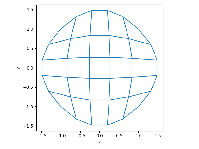
Make the Mesh

Next the mesh would be created. In this case, it was taken to be a convexly deformed square.

N = 6
P = 3

n1 = N
n2 = N


rect_mesh, rx, ry = rmsh.create_elliptical_mesh(
    rmsh.MeshBlock(
        label=None,
        bottom=rmsh.BoundaryCurve.from_knots(n1, (-1, -1), (0, -2), (+1, -1)),
        right=rmsh.BoundaryCurve.from_knots(n2, (+1, -1), (+2, 0), (+1, +1)),
        top=rmsh.BoundaryCurve.from_knots(n2, (+1, +1), (0, +2), (-1, +1)),
        left=rmsh.BoundaryCurve.from_knots(n2, (-1, +1), (-2, 0), (-1, -1)),
    )
)
assert rx < 1e-6 and ry < 1e-6

mesh = Mesh2D(
    P,
    np.stack((rect_mesh.pos_x, rect_mesh.pos_y), axis=-1),
    rect_mesh.lines + 1,
    rect_mesh.surfaces,
)

fig, ax = plt.subplots(1, 1)

xlim, ylim = rect_mesh.plot(ax)
ax.set(
    aspect="equal",
    xlim=(1.1 * xlim[0], 1.1 * xlim[1]),
    ylim=(1.1 * ylim[0], 1.1 * ylim[1]),
    xlabel="$x$",
    ylabel="$y$",
)
fig.tight_layout()
plt.show()

Run Unsteady Simulations

With the mesh and system defined, the simulations can be run. The run is done for 10, 20, 50, 100, and 200 time steps.

nt_vals = np.array((10, 20, 50, 100, 200))
h1_err = np.zeros(nt_vals.size)
l2_err = np.zeros(nt_vals.size)
dt_vals = np.zeros(nt_vals.size)

for i_nt, nt in enumerate(nt_vals):
    dt = float(T_END / nt)
    solutions, stats = solve_system_2d(
        mesh,
        system_settings=SystemSettings(system, initial_conditions={u: initial_u}),
        solver_settings=SolverSettings(
            maximum_iterations=10, relative_tolerance=0, absolute_tolerance=1e-10
        ),
        time_settings=TimeSettings(dt=dt, nt=nt, time_march_relations={v: u}),
        recon_order=25,
    )

    n_sol = len(solutions)
    h1_err_vals = np.zeros(n_sol)
    l2_err_vals = np.zeros(n_sol)
    time_vals = np.zeros(n_sol)

    for isol, sol in enumerate(solutions):
        time = float(sol.field_data["time"][0])

        u_exact = initial_u(sol.points[:, 0], sol.points[:, 1]) * np.exp(
            -ALPHA * time
        ) + final_u(sol.points[:, 0], sol.points[:, 1]) * (1 - np.exp(-ALPHA * time))
        q_exact = initial_q(sol.points[:, 0], sol.points[:, 1]) * np.exp(
            -ALPHA * time
        ) + final_q(sol.points[:, 0], sol.points[:, 1]) * (1 - np.exp(-ALPHA * time))

        u_err = sol.point_data["u"] - u_exact

        q_err = sol.point_data["q"] - q_exact
        sol.point_data["u_err"] = (u_err) ** 2
        # sol.point_data["u_real"] = u_exact
        sol.point_data["q_err"] = np.linalg.norm(q_err, axis=-1)
        # sol.point_data["q_real"] = q_exact

        integrated = sol.integrate_data()
        time_vals[isol] = time
        h1_err_vals[isol] = integrated.point_data["q_err"][0]
        l2_err_vals[isol] = np.sqrt(integrated.point_data["u_err"][0])

    total_h1_error = trapezoid(h1_err_vals, time_vals)
    total_l2_error = trapezoid(l2_err_vals, time_vals)
    h1_err[i_nt] = total_h1_error
    l2_err[i_nt] = total_l2_error
    dt_vals[i_nt] = dt
    # print(f"For {dt=} total error was {total_h1_error:.3e}.")

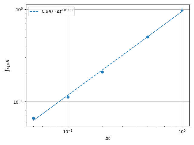
Plot the Time Error

The total integrated time error in the two norms is now examined.

\(H^1\) Norm

k1, k0 = np.polyfit(np.log(dt_vals), np.log(h1_err), 1)
k0 = np.exp(k0)

fig, ax = plt.subplots(1, 1)
ax.scatter(dt_vals, h1_err)
ax.plot(
    dt_vals,
    k0 * dt_vals**k1,
    linestyle="dashed",
    label=f"${k0:.3g} \\cdot {{\\Delta t}}^{{{k1:+.3g}}}$",
)
ax.grid()
ax.legend()
ax.set(
    xlabel="$\\Delta t$",
    ylabel="$\\int \\varepsilon_{H^{1}} {dt}$",
    xscale="log",
    yscale="log",
)
ax.xaxis_inverted()
fig.tight_layout()
plt.show()

\(L^2\) Norm

k1, k0 = np.polyfit(np.log(dt_vals), np.log(l2_err), 1)
k0 = np.exp(k0)

fig, ax = plt.subplots(1, 1)
ax.scatter(dt_vals, l2_err)
ax.plot(
    dt_vals,
    k0 * dt_vals**k1,
    linestyle="dashed",
    label=f"${k0:.3g} \\cdot {{\\Delta t}}^{{{k1:+.3g}}}$",
)
ax.grid()
ax.legend()
ax.set(
    xlabel="$\\Delta t$",
    ylabel="$\\int \\varepsilon_{L^{1}} {dt}$",
    xscale="log",
    yscale="log",
)
ax.xaxis_inverted()
fig.tight_layout()
plt.show()

Plot Solution’s Evolution

With pyvista the unsteady solution can even be plotted.

plotter = pv.Plotter(off_screen=True, window_size=(1600, 800))

plotter.open_gif("unsteady-reaction-direct-solution.gif", fps=30)

for sol in solutions:
    sol.points[:, 2] = sol.point_data["u"]
    plotter.add_mesh(sol, scalars=None, name="solution", show_scalar_bar=False)
    plotter.add_text(f"time = {sol.field_data['time'][0]:.1f}", name="time")
    plotter.write_frame()

plotter.close()