Note
Go to the end to download the full example code.
Mixed Reaction Equation#
Mixed reaction equation examples is exactly the same equation as the one in Reaction Equation, but with the difference being that now \(u\) is taken to be a 2-form instead of a 0-form. As such, there is now a real necessety to introduce a 1-form for its derivative.
import numpy as np
import numpy.typing as npt
import pyvista as pv
import rmsh
from matplotlib import pyplot as plt
from mfv2d import (
    ConvergenceSettings,
    KFormSystem,
    KFormUnknown,
    SolverSettings,
    SystemSettings,
    TimeSettings,
    UnknownFormOrder,
    mesh_create,
    solve_system_2d,
    system_as_string,
)
from scipy.integrate import trapezoid
Setup#
For this case a different initial and final solutions are used as well. For the initial solution given by equation (1) and the final solution given by the equation (2). The primary reason for using these is that because now due to the weak derivative the boundary conditions will be imposed on the solution. Since they can not change in time, these solutions were chosen, as they remain 0 on the boundaries of the domain given by \((x, y) \in [-1, +1] \times [-1, +1]\).
Also, for the value of the reaction coefficient the value of \(\alpha = 1\) is taken. As for the duration, the time slice \(t \in [0, 5]\) was chosen.
ALPHA = 1.0
T_END = 5


def final_u(x: npt.NDArray[np.floating], y: npt.NDArray[np.floating]):
    """Screw initial solution."""
    return (1 - x**4) * (1 - y**4)


def final_q(x: npt.NDArray[np.floating], y: npt.NDArray[np.floating]):
    """Screw initial gradient."""
    return np.stack(
        (
            -4 * x**3 * (1 - y**4),
            -4 * y**3 * (1 - x**4),
        ),
        axis=-1,
    )


def initial_u(x: npt.NDArray[np.floating], y: npt.NDArray[np.floating]):
    """Steady state forcing."""
    return (1 - x**2) * (1 - y**2)


def initial_q(x: npt.NDArray[np.floating], y: npt.NDArray[np.floating]):
    """Steady state gradient."""
    return np.stack(
        (
            -2 * x * (1 - y**2),
            -2 * y * (1 - x**2),
        ),
        axis=-1,
    )
System Setup#
The system setup is about what it was for the direct formulation, except for the second equation pertaining to the gradient of the solution no longer being optional. Since it includes integration by parts, it also includes weak boundary conditions.
u = KFormUnknown("u", UnknownFormOrder.FORM_ORDER_2)
v = u.weight
q = KFormUnknown("q", UnknownFormOrder.FORM_ORDER_1)
p = q.weight

system = KFormSystem(
    ALPHA * (v @ u) == ALPHA * (v @ final_u),
    p.derivative @ u - p @ q == p ^ final_u,
)
print(system_as_string(system))
[M(2)             | 0        ] [u(2)]   [+ E<u, final_u>]   [0 | 0] [u(2)]
[(E(2, 1))^T M(2) | -1.0 M(1)] [q(1)] = [+ B<q, final_u>] + [0 | 0] [q(1)]
Make the Mesh#
As mentioned above, the mesh used for this example is the \((x, y) \in [-1, +1] \times [-1, +1]\) square.
N = 6
P = 4

n1 = N
n2 = N

rect_mesh, rx, ry = rmsh.create_elliptical_mesh(
    rmsh.MeshBlock(
        label=None,
        bottom=rmsh.BoundaryCurve.from_line(n1, (-1, -1), (+1, -1)),
        right=rmsh.BoundaryCurve.from_line(n2, (+1, -1), (+1, +1)),
        top=rmsh.BoundaryCurve.from_line(n2, (+1, +1), (-1, +1)),
        left=rmsh.BoundaryCurve.from_line(n2, (-1, +1), (-1, -1)),
    )
)
assert rx < 1e-6 and ry < 1e-6

mesh = mesh_create(
    P,
    np.stack((rect_mesh.pos_x, rect_mesh.pos_y), axis=-1),
    rect_mesh.lines + 1,
    rect_mesh.surfaces,
)
Run Unsteady Simulations#
With the mesh and system defined, the simulations can be run. The run is done for 10, 20, 50, and 100 time steps.
nt_vals = np.array((10, 20, 50, 100))
h1_err = np.zeros(nt_vals.size)
l2_err = np.zeros(nt_vals.size)
dt_vals = np.zeros(nt_vals.size)

for i_nt, nt in enumerate(nt_vals):
    dt = float(T_END / nt)
    solutions, stats, mesh = solve_system_2d(
        mesh,
        system_settings=SystemSettings(
            system, initial_conditions={u: initial_u, q: initial_q}
        ),
        solver_settings=SolverSettings(
            ConvergenceSettings(
                maximum_iterations=10, relative_tolerance=0, absolute_tolerance=1e-10
            )
        ),
        time_settings=TimeSettings(dt=dt, nt=nt, time_march_relations={v: u}),
        recon_order=10,
    )

    n_sol = len(solutions)
    h1_err_vals = np.zeros(n_sol)
    l2_err_vals = np.zeros(n_sol)
    time_vals = np.zeros(n_sol)

    for isol, sol in enumerate(solutions):
        time = float(sol.field_data["time"][0])

        u_exact = initial_u(sol.points[:, 0], sol.points[:, 1]) * np.exp(
            -ALPHA * time
        ) + final_u(sol.points[:, 0], sol.points[:, 1]) * (1 - np.exp(-ALPHA * time))

        q_exact = initial_q(sol.points[:, 0], sol.points[:, 1]) * np.exp(
            -ALPHA * time
        ) + final_q(sol.points[:, 0], sol.points[:, 1]) * (1 - np.exp(-ALPHA * time))
        u_err = sol.point_data["u"] - u_exact
        q_err = sol.point_data["q"] - q_exact
        sol.point_data["u_err"] = u_err**2
        sol.point_data["q_err"] = np.linalg.norm(q_err, axis=-1)
        sol.point_data["u_real"] = u_exact
        sol.point_data["q_real"] = q_exact

        integrated = sol.integrate_data()
        time_vals[isol] = time
        l2_err_vals[isol] = np.sqrt(integrated.point_data["u_err"][0])
        h1_err_vals[isol] = integrated.point_data["q_err"][0]
        # sol.save(f"sandbox/heat/res-{isol:04d}.vtu")

    h1_total_error = trapezoid(h1_err_vals, time_vals)
    h1_err[i_nt] = h1_total_error
    l2_total_error = trapezoid(l2_err_vals, time_vals)
    l2_err[i_nt] = l2_total_error
    dt_vals[i_nt] = dt
    # print(f"For {dt=} total error was {h1_total_error:.3e}.")
Plot the Time Error#
The total integrated time error in the two norms is now examined.
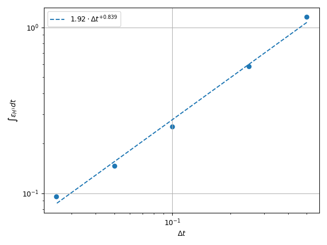
\(H^1\) Norm#
k1, k0 = np.polyfit(np.log(dt_vals), np.log(h1_err), 1)
k0 = np.exp(k0)

fig, ax = plt.subplots(1, 1)
ax.scatter(dt_vals, h1_err)
ax.plot(
    dt_vals,
    k0 * dt_vals**k1,
    linestyle="dashed",
    label=f"${k0:.3g} \\cdot {{\\Delta t}}^{{{k1:+.3g}}}$",
)
ax.grid()
ax.legend()
ax.set(
    xlabel="$\\Delta t$",
    ylabel="$\\int \\varepsilon_{H^{1}} {dt}$",
    xscale="log",
    yscale="log",
)
ax.xaxis_inverted()
fig.tight_layout()
plt.show()
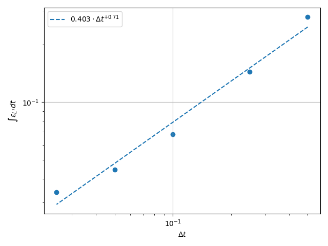
\(L^2\) Norm#
k1, k0 = np.polyfit(np.log(dt_vals), np.log(l2_err), 1)
k0 = np.exp(k0)

fig, ax = plt.subplots(1, 1)
ax.scatter(dt_vals, l2_err)
ax.plot(
    dt_vals,
    k0 * dt_vals**k1,
    linestyle="dashed",
    label=f"${k0:.3g} \\cdot {{\\Delta t}}^{{{k1:+.3g}}}$",
)
ax.grid()
ax.legend()
ax.set(
    xlabel="$\\Delta t$",
    ylabel="$\\int \\varepsilon_{L^{1}} {dt}$",
    xscale="log",
    yscale="log",
)
ax.xaxis_inverted()
fig.tight_layout()
plt.show()
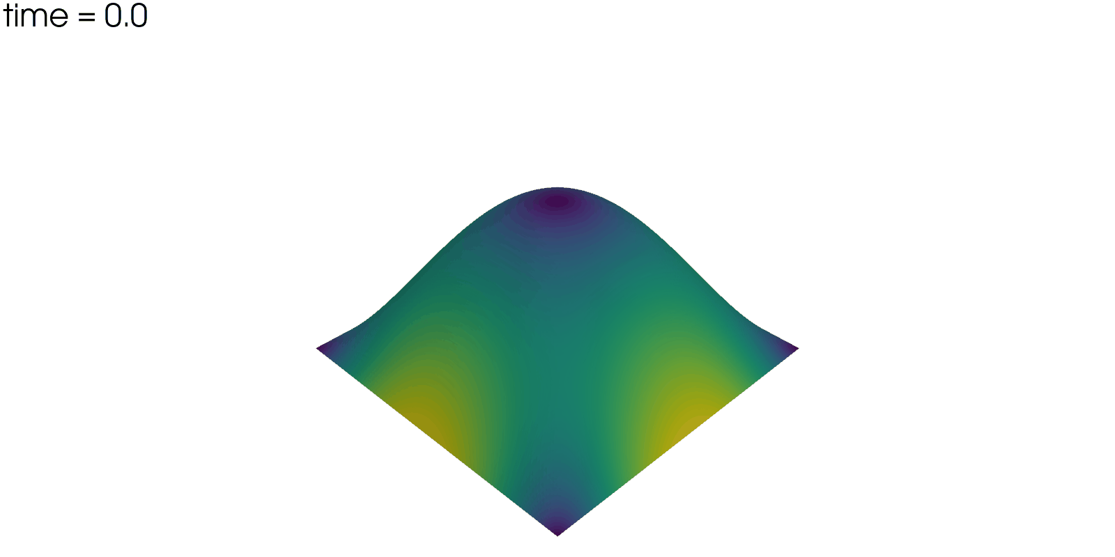
Plot Solution’s Evolution#
With pyvista the unsteady solution can even be plotted.
plotter = pv.Plotter(off_screen=True, window_size=(1600, 800))

plotter.open_gif("unsteady-reaction-mixed-solution.gif", fps=30)

for sol in solutions:
    sol.points[:, 2] = sol.point_data["u"]
    plotter.add_mesh(sol, scalars=None, name="solution", show_scalar_bar=False)
    plotter.add_text(f"time = {sol.field_data['time'][0]:.1f}", name="time")
    plotter.write_frame()

plotter.close()
Total running time of the script: (0 minutes 33.175 seconds)