Unsteady Heat Equations in Mixed Formulation

This example is exactly the same as Unsteady Heat Equations in Direct Formulation. As such, only differences from that one will be mentioned.

import numpy as np
import numpy.typing as npt
import rmsh
from matplotlib import pyplot as plt
from mfv2d import (
    KFormSystem,
    KFormUnknown,
    Mesh2D,
    SolverSettings,
    SystemSettings,
    TimeSettings,
    UnknownFormOrder,
    solve_system_2d,
)
from scipy.integrate import trapezoid

Setup

Since the mixed formulation naturally also gives the graident, it is also computed here.

ALPHA = 0.02
BETA = 1


def steady_u(x: npt.NDArray[np.floating], y: npt.NDArray[np.floating]):
    """Steady state solution."""
    return np.cos(np.pi * x / 2) * np.cos(np.pi * y / 2)


def steady_q(x: npt.NDArray[np.floating], y: npt.NDArray[np.floating]):
    """Steady state gradient."""
    return np.stack(
        (
            -np.pi / 2 * np.sin(np.pi * x / 2) * np.cos(np.pi * y / 2),
            -np.pi / 2 * np.cos(np.pi * x / 2) * np.sin(np.pi * y / 2),
        ),
        axis=-1,
    )


u = KFormUnknown("u", UnknownFormOrder.FORM_ORDER_2)
v = u.weight
q = KFormUnknown("q", UnknownFormOrder.FORM_ORDER_1)
p = q.weight

system = KFormSystem(
    p.derivative * u - p * q == p ^ steady_u,
    ALPHA * (v * q.derivative)
    == BETA * (v * steady_u) - (BETA - ALPHA * np.pi**2 / 2) * (v * u),
    sorting=lambda f: f.order,
)
print(system)

N = 13
P = 3
T_END = 2

n1 = N
n2 = N
rect_mesh, rx, ry = rmsh.create_elliptical_mesh(
    rmsh.MeshBlock(
        label=None,
        bottom=rmsh.BoundaryCurve.from_line(n1, (-1, -1), (+1, -1)),
        right=rmsh.BoundaryCurve.from_line(n2, (+1, -1), (+1, +1)),
        top=rmsh.BoundaryCurve.from_line(n2, (+1, +1), (-1, +1)),
        left=rmsh.BoundaryCurve.from_line(n2, (-1, +1), (-1, -1)),
    )
)
assert rx < 1e-6 and ry < 1e-6
mesh = Mesh2D(
    P,
    np.stack((rect_mesh.pos_x, rect_mesh.pos_y), axis=-1),
    rect_mesh.lines + 1,
    rect_mesh.surfaces,
)

nt_vals = np.logspace(start=1, stop=5, num=6, base=2, dtype=np.uint32)
h1_err = np.zeros(nt_vals.size)
l2_err = np.zeros(nt_vals.size)
dt_vals = np.zeros(nt_vals.size)

for i_nt, nt in enumerate(nt_vals):
    dt = float(T_END / nt)
    solutions, stats = solve_system_2d(
        mesh,
        system_settings=SystemSettings(system),
        solver_settings=SolverSettings(
            maximum_iterations=20, relative_tolerance=0, absolute_tolerance=1e-13
        ),
        time_settings=TimeSettings(dt=dt, nt=nt, time_march_relations={v: u}),
        recon_order=25,
    )

    n_sol = len(solutions)
    h1_vals = np.zeros(n_sol)
    l2_vals = np.zeros(n_sol)
    time_vals = np.zeros(n_sol)
    for isol, sol in enumerate(solutions):
        time = float(sol.field_data["time"][0])

        u_exact = steady_u(sol.points[:, 0], sol.points[:, 1]) * (
            1 - np.exp(-BETA * time)
        )
        u_err = sol.point_data["u"] - u_exact
        sol.point_data["u_err"] = u_err**2
        sol.point_data["u_exact"] = u_exact

        q_exact = steady_q(sol.points[:, 0], sol.points[:, 1]) * (
            1 - np.exp(-BETA * time)
        )
        q_err = sol.point_data["q"] - q_exact
        sol.point_data["q_err"] = np.linalg.norm(q_err, axis=-1)
        sol.point_data["q_exact"] = q_exact

        integrated = sol.integrate_data()
        time_vals[isol] = time
        h1_vals[isol] = integrated.point_data["q_err"][0]
        l2_vals[isol] = np.sqrt(integrated.point_data["u_err"])[0]
        # print(f"Error at time {time:.3g} is {err:.3e}")

    h1_total_error = trapezoid(h1_vals, time_vals)
    l2_total_error = trapezoid(l2_vals, time_vals)
    h1_err[i_nt] = h1_total_error
    l2_err[i_nt] = l2_total_error
    dt_vals[i_nt] = dt
    print(f"For {dt=:.3g} total error was {h1_total_error:.3e}.")

[q(2*)]^T  ([            -1 * M(2) | (E(3, 2))^T @ M(2)]  [q(1)]   [<q, steady_u>])   [q(2*)]^T  ([0 |                0]  [q(1)]
[u(3*)]    ([0.02 * M(3) @ E(3, 2) |                  0]  [u(2)] = [<u, steady_u>]) + [u(3*)]    ([0 | -0.901304 * M(3)]  [u(2)]
For dt=1 total error was 1.986e-01.
For dt=0.667 total error was 9.133e-02.
For dt=0.333 total error was 2.327e-02.
For dt=0.2 total error was 8.415e-03.
For dt=0.111 total error was 2.613e-03.
For dt=0.0625 total error was 8.619e-04.

Plotting the Error

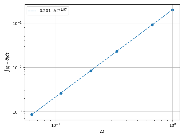
Now we plot the error. As you can see, we magically got another order of accuracy out of fucking thin air. If I had to guess it is related to the fact that the time integration is symplectic.

\(H^1\) Norm

k1, k0 = np.polyfit(np.log(dt_vals), np.log(h1_err), 1)
k0 = np.exp(k0)

fig, ax = plt.subplots(1, 1)
ax.scatter(dt_vals, h1_err)
ax.plot(
    dt_vals,
    k0 * dt_vals**k1,
    linestyle="dashed",
    label=f"${k0:.3g} \\cdot {{\\Delta t}}^{{{k1:+.3g}}}$",
)
ax.grid()
ax.legend()
ax.set(
    xlabel="$\\Delta t$",
    ylabel="$\\int \\left|q - \\bar{q}\\right| {dt}$",
    xscale="log",
    yscale="log",
)
ax.xaxis_inverted()
fig.tight_layout()
plt.show()

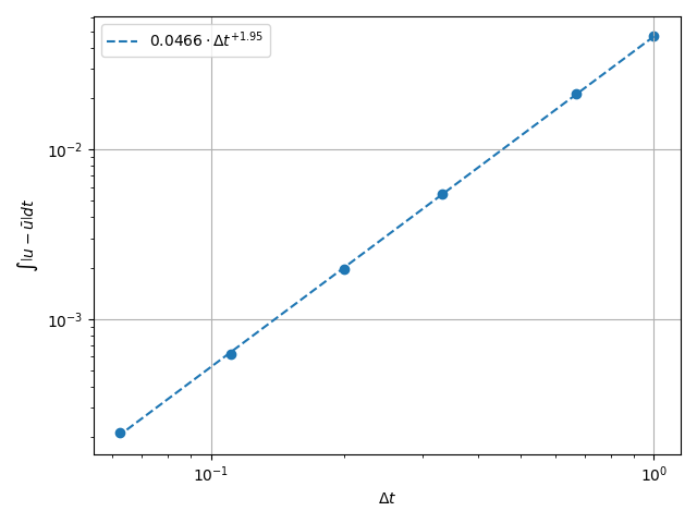
\(L^2\) Norm

k1, k0 = np.polyfit(np.log(dt_vals), np.log(l2_err), 1)
k0 = np.exp(k0)

fig, ax = plt.subplots(1, 1)
ax.scatter(dt_vals, l2_err)
ax.plot(
    dt_vals,
    k0 * dt_vals**k1,
    linestyle="dashed",
    label=f"${k0:.3g} \\cdot {{\\Delta t}}^{{{k1:+.3g}}}$",
)
ax.grid()
ax.legend()
ax.set(
    xlabel="$\\Delta t$",
    ylabel="$\\int \\left|u - \\bar{u}\\right| {dt}$",
    xscale="log",
    yscale="log",
)
ax.xaxis_inverted()
fig.tight_layout()
plt.show()