Note
Go to the end to download the full example code.
Vector Reaction Equation#
Vector reaction equation examples is solving the same equations as Reaction Equation and Mixed Reaction Equation, but with the \(u\) being a 1-form. This does just makes the solution have two decoupled components, which are solved for independently.
import numpy as np
import numpy.typing as npt
import rmsh
from matplotlib import pyplot as plt
from mfv2d import (
    ConvergenceSettings,
    KFormSystem,
    KFormUnknown,
    SolverSettings,
    SystemSettings,
    TimeSettings,
    UnknownFormOrder,
    mesh_create,
    solve_system_2d,
)
from scipy.integrate import trapezoid
Setup#
For this case a initial and final solutions are given by equations (1) and (2) respectivly.
As for the value of the reaction coefficient and the time slice, the value of \(\alpha = 0.5\) and the time slice \(t \in [0, 5]\) were chosen.
ALPHA = 0.5
T_END = 5


def initial_u(x: npt.NDArray[np.floating], y: npt.NDArray[np.floating]):
    """Screw initial solution."""
    return np.stack((2 * x * y, x**2 * y), axis=-1)


def final_u(x: npt.NDArray[np.floating], y: npt.NDArray[np.floating]):
    """Steady state solution."""
    return np.stack(
        (
            -(x**2) * y,
            -x * y,
        ),
        axis=-1,
    )
System Setup#
The system setup the same as for other reaction equations. The only difference is that for this case no second equation for the gradients were introduced.
u = KFormUnknown("u", UnknownFormOrder.FORM_ORDER_1)
v = u.weight

system = KFormSystem(
    ALPHA * (v @ u) == ALPHA * (v @ final_u),
    sorting=lambda f: f.order,
)
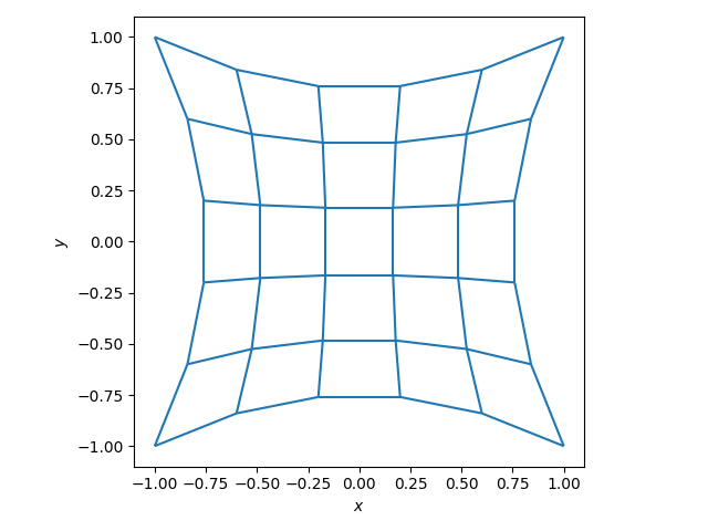
Make the Mesh#
Next the mesh would be created. In this case, it was taken to be a concavely deformed square.
N = 6
P = 4

n1 = N
n2 = N
rect_mesh, rx, ry = rmsh.create_elliptical_mesh(
    rmsh.MeshBlock(
        label=None,
        bottom=rmsh.BoundaryCurve.from_knots(n1, (-1, -1), (0, -0.5), (+1, -1)),
        right=rmsh.BoundaryCurve.from_knots(n2, (+1, -1), (+0.5, 0), (+1, +1)),
        top=rmsh.BoundaryCurve.from_knots(n2, (+1, +1), (0, +0.5), (-1, +1)),
        left=rmsh.BoundaryCurve.from_knots(n2, (-1, +1), (-0.5, 0), (-1, -1)),
    )
)
assert rx < 1e-6 and ry < 1e-6

mesh = mesh_create(
    P,
    np.stack((rect_mesh.pos_x, rect_mesh.pos_y), axis=-1),
    rect_mesh.lines + 1,
    rect_mesh.surfaces,
)

fig, ax = plt.subplots(1, 1)

xlim, ylim = rect_mesh.plot(ax)
ax.set(
    aspect="equal",
    xlim=(1.1 * xlim[0], 1.1 * xlim[1]),
    ylim=(1.1 * ylim[0], 1.1 * ylim[1]),
    xlabel="$x$",
    ylabel="$y$",
)
fig.tight_layout()
plt.show()
Run Unsteady Simulations#
With the mesh and system defined, the simulations can be run. The run is done for 10, 20, 50, and 100 time steps.
nt_vals = np.array((10, 20, 50, 100))
l2_err = np.zeros(nt_vals.size)
dt_vals = np.zeros(nt_vals.size)

for i_nt, nt in enumerate(nt_vals):
    dt = float(T_END / nt)
    solutions, stats, mesh = solve_system_2d(
        mesh,
        system_settings=SystemSettings(system, initial_conditions={u: initial_u}),
        solver_settings=SolverSettings(
            ConvergenceSettings(
                maximum_iterations=10, relative_tolerance=0, absolute_tolerance=1e-10
            )
        ),
        time_settings=TimeSettings(dt=dt, nt=nt, time_march_relations={v: u}),
        recon_order=10,
    )

    n_sol = len(solutions)
    l2_err_vals = np.zeros(n_sol)
    time_vals = np.zeros(n_sol)

    for isol, sol in enumerate(solutions):
        time = float(sol.field_data["time"][0])

        u_exact = initial_u(sol.points[:, 0], sol.points[:, 1]) * np.exp(
            -ALPHA * time
        ) + final_u(sol.points[:, 0], sol.points[:, 1]) * (1 - np.exp(-ALPHA * time))

        u_err = sol.point_data["u"] - u_exact

        sol.point_data["u_err"] = np.linalg.norm(u_err, axis=-1)
        sol.point_data["u_real"] = u_exact

        integrated = sol.integrate_data()
        err = float(integrated.point_data["u_err"][0])
        time_vals[isol] = time
        l2_err_vals[isol] = err

    total_time_error = trapezoid(l2_err_vals, time_vals)
    l2_err[i_nt] = total_time_error
    dt_vals[i_nt] = dt
    print(f"For {dt=} total error was {total_time_error:.3e}.")
For dt=0.5 total error was 2.608e-01.
For dt=0.25 total error was 1.334e-01.
For dt=0.1 total error was 5.407e-02.
For dt=0.05 total error was 2.715e-02.
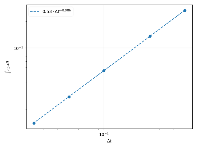
Plot the Time Error#
The total integrated time error in the two norms is now examined.
k1, k0 = np.polyfit(np.log(dt_vals), np.log(l2_err), 1)
k0 = np.exp(k0)

fig, ax = plt.subplots(1, 1)
ax.scatter(dt_vals, l2_err)
ax.plot(
    dt_vals,
    k0 * dt_vals**k1,
    linestyle="dashed",
    label=f"${k0:.3g} \\cdot {{\\Delta t}}^{{{k1:+.3g}}}$",
)
ax.grid()
ax.legend()
ax.set(
    xlabel="$\\Delta t$",
    ylabel="$\\int \\varepsilon_{L^{1}} {dt}$",
    xscale="log",
    yscale="log",
)
ax.xaxis_inverted()
fig.tight_layout()
plt.show()
Total running time of the script: (0 minutes 2.694 seconds)