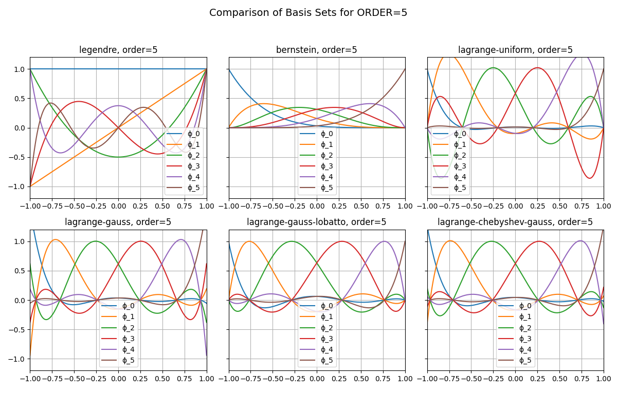
Basis Sets Visualization

This example demonstrates how different basis sets look for polynomial orders. We compare Lagrange, Legendre, and Bernstein-type bases using different node distributions (uniform, Gauss, Gauss-Lobatto, Chebyshev-Gauss).

The basis values are sampled at the integration points (nodes), and the functions are visualized on the reference interval [-1, 1].

# Assume classes are defined in fdg
import numpy as np
from fdg import BasisSpecs, BasisType
from matplotlib import pyplot as plt
from matplotlib.axes import Axes

Helper function to plot a basis set

def plot_basis_set(basis_type: BasisType, order: int, ax: Axes) -> None:
    """Plot basis in the set."""
    basis_specs = BasisSpecs(basis_type, order)

    x = np.linspace(-1, +1, 200)
    v = basis_specs.values(x)

    for i in range(v.shape[-1]):
        ax.plot(x, v[..., i], label=f"ϕ_{i}")
    ax.set_title(f"{basis_type.value}, order={order}")
    ax.set_xlim(-1, +1)
    ax.set_ylim(-1.2, +1.2)
    ax.legend()
    ax.grid(True)


def plot_basis_set_derivatives(basis_type: BasisType, order: int, ax: Axes) -> None:
    """Plot basis derivatives in the set."""
    basis_specs = BasisSpecs(basis_type, order)

    x = np.linspace(-1, +1, 200)
    v = basis_specs.derivatives(x)

    for i in range(v.shape[-1]):
        ax.plot(x, v[..., i], label=f"ϕ_{i}")
    ax.set_title(f"{basis_type.value}, order={order}")
    ax.set_xlim(-1, +1)
    ax.set_ylim(-2, +2)
    ax.legend()
    ax.grid(True)

Specify Config

ORDER = 5

Compare different basis types

fig, axes = plt.subplots(2, 3, figsize=(12, 8), sharey=True)


for ax, btype in zip(axes.flat, BasisType):
    plot_basis_set(BasisType(btype), order=ORDER, ax=ax)

fig.suptitle(f"Comparison of Basis Sets for {ORDER=}", fontsize=14)

fig.tight_layout(rect=(0, 0.05, 1, 0.95))
# plt.show()

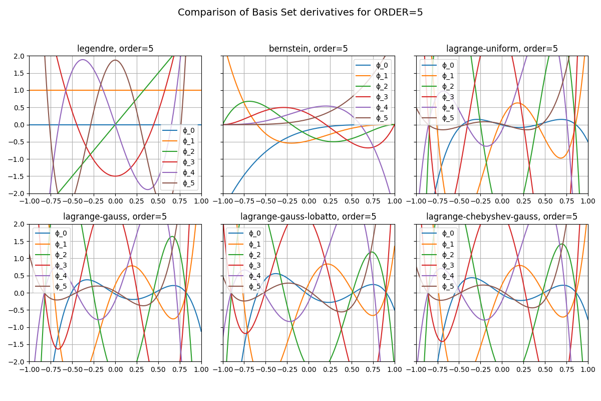
Compare derivatives of different basis types

fig, axes = plt.subplots(2, 3, figsize=(12, 8), sharey=True)

for ax, btype in zip(axes.flat, BasisType):
    plot_basis_set_derivatives(BasisType(btype), order=ORDER, ax=ax)

fig.suptitle(f"Comparison of Basis Set derivatives for {ORDER=}", fontsize=14)

fig.tight_layout(rect=(0, 0.05, 1, 0.95))
plt.show()