Integration Rules

This example is intended to showcase how integration rules work. There are currently two supported rules:

• "gauss", which is uses Gaussian quadrature,

• "gauss-lobatto", which is uses Gaussian-Lobbato-Legendre nodes for quadrature.

import numpy as np
from fdg import IntegrationMethod, IntegrationSpecs
from matplotlib import pyplot as plt

Different Types of Integration Rules

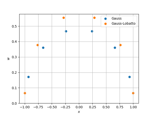
There are different types of integration rules. The first one is the Gaussian quadrature, which is accurate up to the integrals of order \(2n - 1\) for a rule of order \(n\). The second one is the Gauss-Lobatto quadrature, which also includes the endpoints of the domain, which makes it useful for some cases, but it reduces the accuracy of integration to order \(2n - 3\) for a rule of order \(n\).

rule_gauss = IntegrationSpecs(5, IntegrationMethod.GAUSS)
rule_gl = IntegrationSpecs(5, IntegrationMethod.GAUSS_LOBATTO)

fig, ax = plt.subplots()
ax.scatter(rule_gauss.nodes(), rule_gauss.weights(), label="Gauss")
ax.scatter(rule_gl.nodes(), rule_gl.weights(), label="Gauss-Lobatto")
ax.grid()
ax.legend()
ax.set_ylim(0)
ax.set(xlabel="$x$", ylabel="$w$")
plt.show()

Integrating Polynomials

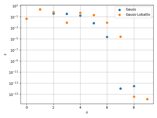
Polynomials are exactly integrated up to the degree which is given by the IntegrationRule.accuracy property. The error decreases exponentially as that order is approached.

rng = np.random.default_rng(seed=0)  # Make rng predictable
N_POLY = 14
coeffs = rng.uniform(0, 1, size=N_POLY + 1)
poly = np.polynomial.Legendre(coeffs, domain=(-1, +1))

Using Gaussian Quadrature

gauss_integral_values: list[float] = list()

gauss_order = 0
while True:
    rule = IntegrationSpecs(gauss_order, IntegrationMethod.GAUSS)
    value = np.dot(rule.weights(), poly((rule.nodes() - 1) / 2)) / 2
    gauss_integral_values.append(value)
    if rule.accuracy >= N_POLY + 2:
        # Go one further
        break
    gauss_order += 1

Using Gaussian-Lobatto Quadrature

gauss_lobatto_integral_values: list[float] = list()

gauss_lobatto_order = 0
while True:
    rule = IntegrationSpecs(gauss_lobatto_order, IntegrationMethod.GAUSS_LOBATTO)
    value = np.dot(rule.weights(), poly((rule.nodes() - 1) / 2)) / 2
    gauss_lobatto_integral_values.append(value)
    if rule.accuracy >= N_POLY + 2:
        # Go one further
        break
    gauss_lobatto_order += 1


fig, ax = plt.subplots()

ax.scatter(
    np.arange(gauss_order),
    np.abs(
        (np.array(gauss_integral_values[:-1]) - gauss_integral_values[-1])
        / gauss_integral_values[-1]
    ),
    label="Gauss",
)
ax.scatter(
    np.arange(gauss_lobatto_order),
    np.abs(
        (np.array(gauss_lobatto_integral_values[:-1]) - gauss_lobatto_integral_values[-1])
        / gauss_lobatto_integral_values[-1]
    ),
    label="Gauss-Lobatto",
)
ax.set(yscale="log", xlabel="$n$", ylabel="$\\epsilon$")
ax.grid()
ax.legend()
fig.tight_layout()
plt.show()