Note
Go to the end to download the full example code.
Gradients#
import numpy as np
from fdg import (
    BasisSpecs,
    BasisType,
    FunctionSpace,
    IntegrationSpace,
    IntegrationSpecs,
    Line,
    Quad,
    projection_l2_primal,
)
from fdg._fdg import (
    DegreesOfFreedom,
    compute_gradient_mass_matrix,
    compute_mass_matrix,
)
from fdg.degrees_of_freedom import reconstruct
from fdg.enum_type import IntegrationMethod
from matplotlib import pyplot as plt
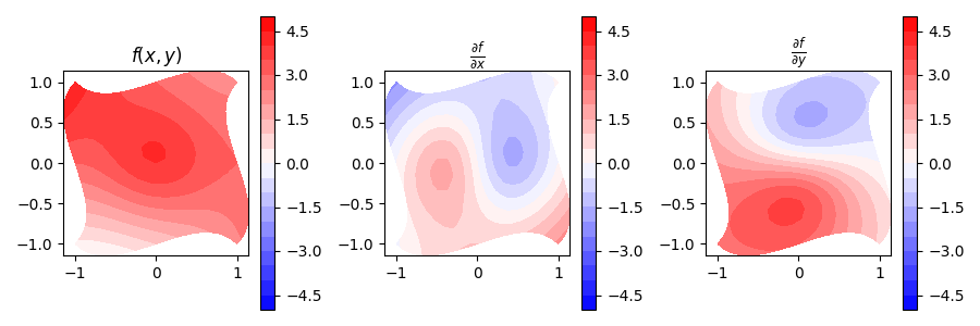
The first thing should be to define a domain. This domain defines the mapping between the reference space, which goes from -1 to +1 for every dimension, to a physical space.
It is possible to have the physical space be of a higher dimension, such as when a 2D domain is mapped to a surface in a 3D space. This example keeps things nice and simple and uses a 2D to 2D mapping.
domain = Quad(
    bottom=Line((-1, -1), (-0.5, -1.5), (+0.5, -0.5), (+1, -1)),
    right=Line((+1, -1), (+1.5, -0.5), (+0.5, +0.5), (+1, +1)),
    top=Line((+1, +1), (+0.5, +1.5), (-0.5, +0.5), (-1, +1)),
    left=Line((-1, +1), (-1.5, +0.5), (-0.5, -0.5), (-1, -1)),
)

s1, s2 = np.meshgrid(np.linspace(-1, +1, 21), np.linspace(-1, +1, 21))
x, y = domain.sample(s1, s2)


def test_function(*args):
    """Example test function."""
    x, y = args
    return x**2 + y * (1 - x) + 4 / (x**2 + y**2 + 1)


def test_function_dx(*args):
    """Analytical x-gradient of the function."""
    x, y = args
    return 2 * x - y - 4 / (x**2 + y**2 + 1) ** 2 * 2 * x


def test_function_dy(*args):
    """Analytical y-gradient of the function."""
    x, y = args
    return 1 - x - 4 / (x**2 + y**2 + 1) ** 2 * 2 * y


fig, (ax_fn, ax_dx, ax_dy) = plt.subplots(nrows=1, ncols=3, figsize=(9, 3))

cp = ax_fn.contourf(x, y, test_function(x, y), levels=np.linspace(-5, +5, 21), cmap="bwr")
fig.colorbar(cp)
ax_fn.set(aspect="equal", title="$f(x, y)$")

cp = ax_dx.contourf(
    x, y, test_function_dx(x, y), levels=np.linspace(-5, +5, 21), cmap="bwr"
)
fig.colorbar(cp)
ax_dx.set(aspect="equal", title="$\\frac{ \\partial f }{ \\partial x }$")


cp = ax_dy.contourf(
    x, y, test_function_dy(x, y), levels=np.linspace(-5, +5, 21), cmap="bwr"
)
fig.colorbar(cp)
ax_dy.set(aspect="equal", title="$\\frac{ \\partial f }{ \\partial y }$")

fig.tight_layout()
plt.show()
We first pick a function space in which the function will be represented.
N = 5

func_space = FunctionSpace(
    BasisSpecs(BasisType.LEGENDRE, N),
    BasisSpecs(BasisType.LEGENDRE, N),
)
To be able to compute an \(L^2\) projection of anything onto this function space, we first need an integration space. In this case, we use over-integration, meaning that the order of integration is high enough to fully resolve all polynomials correctly.
This integration space is only valid on the reference domain. As such, it has to be associated with a coordinate mapping which makes up the map from reference space to physical space.
space_map = domain(int_space)

func_proj = projection_l2_primal(test_function, func_space, space_map)

s1, s2 = np.meshgrid(np.linspace(-1, +1, 51), np.linspace(-1, +1, 51))
x, y = domain.sample(s1, s2)

f_recon = reconstruct(func_proj, s1, s2)
f_real = test_function(x, y)

fig, (ax_fn, ax_proj, ax_err) = plt.subplots(nrows=1, ncols=3, figsize=(9, 3))
# Plot the function
cp = ax_fn.contourf(x, y, f_real, levels=np.linspace(-5, +5, 21), cmap="bwr")
fig.colorbar(cp)
ax_fn.set(aspect="equal", title="$f(x, y)$")

cp = ax_proj.contourf(x, y, f_recon, levels=np.linspace(-5, +5, 21), cmap="bwr")
fig.colorbar(cp)
ax_proj.set(aspect="equal", title="$\\overline{ f }(x, y)$")

err = np.abs(f_recon - f_real)
print(f"Min-Max error is: {err.min():4.2g} and {err.max():4.2g}")
cp = ax_err.contourf(x, y, err, norm="log", cmap="magma", levels=np.logspace(-4, 0, 9))
fig.colorbar(cp)
ax_err.set(aspect="equal", title="$\\left| f - \\overline{ f } \\right|$")

fig.tight_layout()
plt.show()
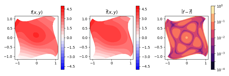
Min-Max error is: 7.3e-05 and 0.15
Derivatives#
Derivatives can also be obtained from projections. What should be noted is that these can only be taken along reference directions, so for derivatives in physical space their components need to be assembled.
Since this example has 2 reference dimensions mapped to 2 physical dimensions, there will be four terms in total. This is because each of the 2 reference derivatives contributes to each of the 2 physical derivatives.
Very important thing to note is that since taking a derivative means that the resulting derivative is one order lower, since polynomial basis are used. As such, it can only have a unique representation in a function space, which is one order lower in that dimension.
# Spaces with lower orders
der0_space = func_space.lower_order(0)  # Function space for derivatives of 1st component
der1_space = func_space.lower_order(1)  # Function space for derivatives of 2nd component

# Needed to transfer dual -> primal
mass0 = compute_mass_matrix(der0_space, der0_space, space_map)
mass1 = compute_mass_matrix(der1_space, der1_space, space_map)

# Contribution of 1st reference component to 1st physical derivative
grad00_mat = compute_gradient_mass_matrix(func_space, der0_space, space_map, 0, 0)
# Contribution of 1st reference component to 2nd physical derivative
grad01_mat = compute_gradient_mass_matrix(func_space, der0_space, space_map, 0, 1)
# Contribution of 2nd reference component to 1st physical derivative
grad10_mat = compute_gradient_mass_matrix(func_space, der1_space, space_map, 1, 0)
# Contribution of 2nd reference component to 2nd physical derivative
grad11_mat = compute_gradient_mass_matrix(func_space, der1_space, space_map, 1, 1)

# Make them dual -> primal operators
grad00_mat = np.linalg.solve(mass0, grad00_mat)
grad01_mat = np.linalg.solve(mass0, grad01_mat)
grad10_mat = np.linalg.solve(mass1, grad10_mat)
grad11_mat = np.linalg.solve(mass1, grad11_mat)
With the operators prepared, we can create degrees of freedom of derivatives.
# Derivative with respect to x
dfdx0_dofs = DegreesOfFreedom(der0_space, grad00_mat @ func_proj.values.flatten())
dfdx1_dofs = DegreesOfFreedom(der1_space, grad10_mat @ func_proj.values.flatten())

# Derivative with respect to y
dfdy0_dofs = DegreesOfFreedom(der0_space, grad01_mat @ func_proj.values.flatten())
dfdy1_dofs = DegreesOfFreedom(der1_space, grad11_mat @ func_proj.values.flatten())
Comparing Reconstructed Derivatives#
We can now check how these derivatives look.
dfdx_recon = reconstruct(dfdx0_dofs, s1, s2) + reconstruct(dfdx1_dofs, s1, s2)
dfdx_real = test_function_dx(x, y)

fig, (ax_fn, ax_proj, ax_err) = plt.subplots(nrows=1, ncols=3, figsize=(9, 3))
# Plot the function
cp = ax_fn.contourf(x, y, dfdx_real, levels=np.linspace(-5, +5, 21), cmap="bwr")
fig.colorbar(cp)
ax_fn.set(aspect="equal", title="$\\frac{ \\mathrm{ d } f } {\\mathrm{ d } x } (x, y)$")

cp = ax_proj.contourf(x, y, dfdx_recon, levels=np.linspace(-5, +5, 21), cmap="bwr")
fig.colorbar(cp)
ax_proj.set(
    aspect="equal",
    title="$\\frac{ \\mathrm{ d } \\overline{ f } } {\\mathrm{ d } x } (x, y)$",
)

err = np.abs(dfdx_recon - dfdx_real)
print(f"Min-Max error is: {err.min():4.2g} and {err.max():4.2g}")
cp = ax_err.contourf(x, y, err, norm="log", cmap="magma", levels=np.logspace(-4, 1, 11))
fig.colorbar(cp)
ax_err.set(
    aspect="equal",
    title=(
        "$\\left| \\frac{ \\mathrm{ d } f } {\\mathrm{ d } x } - "
        "\\frac{ \\mathrm{ d } \\overline{ f } } {\\mathrm{ d } x } \\right|$"
    ),
)

fig.tight_layout()
plt.show()
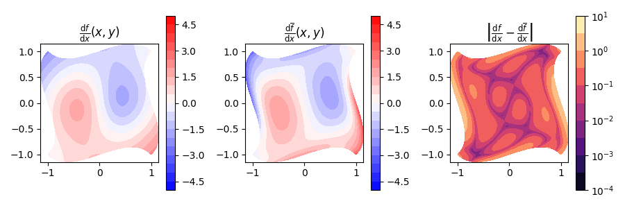
Min-Max error is: 1.6e-15 and 2.8
Now also for the y-derivative.
dfdy_recon = reconstruct(dfdy0_dofs, s1, s2) + reconstruct(dfdy1_dofs, s1, s2)
dfdy_real = test_function_dy(x, y)

fig, (ax_fn, ax_proj, ax_err) = plt.subplots(nrows=1, ncols=3, figsize=(9, 3))
# Plot the function
cp = ax_fn.contourf(x, y, dfdy_real, levels=np.linspace(-5, +5, 21), cmap="bwr")
fig.colorbar(cp)
ax_fn.set(aspect="equal", title="$\\frac{ \\mathrm{ d } f } {\\mathrm{ d } y } (x, y)$")

cp = ax_proj.contourf(x, y, dfdy_recon, levels=np.linspace(-5, +5, 21), cmap="bwr")
fig.colorbar(cp)
ax_proj.set(
    aspect="equal",
    title="$\\frac{ \\mathrm{ d } \\overline{ f } } {\\mathrm{ d } y } (x, y)$",
)

err = np.abs(dfdy_recon - dfdy_real)
print(f"Min-Max error is: {err.min():4.2g} and {err.max():4.2g}")
cp = ax_err.contourf(x, y, err, norm="log", cmap="magma", levels=np.logspace(-4, 1, 11))
fig.colorbar(cp)
ax_err.set(
    aspect="equal",
    title=(
        "$\\left| \\frac{ \\mathrm{ d } f } {\\mathrm{ d } y } - "
        "\\frac{ \\mathrm{ d } \\overline{ f } } {\\mathrm{ d } y } \\right|$"
    ),
)

fig.tight_layout()
plt.show()
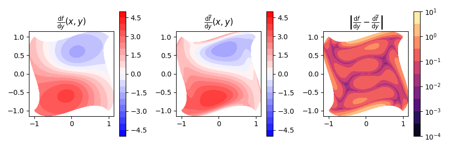
Min-Max error is: 8.9e-16 and 3
Total running time of the script: (0 minutes 1.378 seconds)